Cover page
Student name: John C Gibson
Course number: PHYS.1410L , Section 811
Instructor name: Benjamin MacConnell
Date of experiment: Nov 8, 2023
Partner’s name: (No partner)
Title of experiment:
Impulse and Momentum in Collisions
Objective: Measure an object’s momentum change during collisions by measuring velocity and force. The collision characteristics will be categorized both by velocity and by force measurements.

Introduction
A collision, when no deformation in the object of calculation, is fundamentally a net force acting on that object. Newton’s second law can fully describe the displacement and velocity of the object behaving during the force’s action, and hence the behavior upon the collision. For example, as illustrated in the velocity-time plot, when a constant net force pushes an objection in the opposite direction of its initial velocity v0, and the net force stops when velocity reaches 0.
Fnet=ma
For this special case,
a= slope=(0-v0)/(t1-t0)= -v0/(t1-t0)
t0t1Fnetdt=t0t1madt=mat0t1dt=ma(t1-t0)= -mv0
= rectangle area under constant force Fnet
.
Momentum is defined as p=mv, so
t0t1Fnetdt= -mv0= -p0
, which means that the force integral over time is the momentum of the original object before collision in this special case.
When friction and g forces are included,
Fnet=(Fg+Fk+Fspring)
. The source components of Fnet can be varying, but the integral of Fnet over time equation is still true, t0t1Fnetdt= -mv0= -p0
. Fnet covers all forces summation, but not all forces can be practically measured during an experiment, such as friction and molecular level compression and stretching of the object or force gauge.
Derivation for the general case:
The integral of force over time, when applied to non-constant net force, still equals the area under the Fnet curve, as depicted here on the right because
titfFnetdt = rectangle area under Fnetcurve
, by definition.
When we use the definition of acceleration a=dv/dt in the integration, with calculus variable substitution,
titfFnetdt=titf(mdv/dt)dt=mtitfdv=mvf-mvi
, and reapply p=mv, we get
titfFnetdt=pf-pi= Δp
. For convenience, we define Δp=impulse=J=titfFnetdt .
In this experiment, we have 3 different setups for Vf, in the following 3 sections,
Vf final velocity to be roughly equal to Vi’s magnitude, but velocities in opposite directions.
Vf final velocity to be roughly equal to zero.
Vf final velocity to be smaller than Vi’s magnitude but not equal to zero.
In data recording, mvf-mviwill be recorded as Δp ; % difference will be
(Δp - integral value J)/AVERAGE(J,Δp) * 100 ,
, where the AVERAGE function is (J+Δp)/2 .
Steps
Start by setting up the wireless/wired connection between the computer program and force gauge and displacement detector.
For section A. Vf final velocity to be roughly equal to Vi’s magnitude by using a light spring.
Place the ramp flat on the bench.
Screw on the light spring to the stop fixture.
Place the cart with force gauge in the middle of the ramp.
Click Start button in the data acquisition window.
Gently push the cart assembly from the middle of the ramp toward the spring stop. Make sure the light spring is not pressed to the very limit of the spring.
The data acquisition stops after 5 seconds with a recorded velocity and force plot.
In the velocity window pane, click the Zoom button to narrow down the data points to include the collision where velocity goes from positive Vi to negative Vf final velocity is roughly equal in magnitude but oppositive signs.
In the velocity window pane, click the Statistics button and drag the black brackets the the collision time course. Record the Vf and Vi values.
In the force window pane, click the Integrate button and drag the black brackets to the same collision time course interval. Record the Integrated value of force over time.
In the force window, move the cursor to the trough of the force curve and record the maximum force that is displayed in the bottom left corner.
Repeat from step 3 of this section two more times to obtain 3 data entries for this section of the experiment.
Remove the spring stop.
For section B. Vf final velocity to be roughly equal to zero.
Place the ramp’s head end on the 10cm x 10 cm x 3cm wood block.
Open the small Ziplock bag with a 3cm opening, sealing the rest of the seal. Squeeze the 3cm opening to form a round opening and blow air into the bag to inflate it.
Place the bag at the stop fixture wall in place of the previous spring stop.
Place the cart with a force gauge near the middle of the ramp. Record the distance as the small distance for a small initial Vi velocity.
Click the Start button in the data acquisition window.
Release the cart assembly from the middle of the ramp toward the spring stop. Make sure the airbag is not entirely deflated at the end of the collision course. The velocity curve should be smooth and approach zero at the end of the collision course in the velocity window pane.
The data acquisition stops after 5 seconds with a recorded velocity and force plot.
In the velocity window pane, click the Zoom button to narrow down the data points to include the collision where velocity goes from positive Vi to negative Vf final velocity is roughly equal in magnitude but oppositive signs.
In the velocity window pane, click the Statistics button and drag the black brackets the the collision time course. Record the Vf and Vi values.
In the force window pane, click the Integrate button and drag the black brackets to the same collison time course interval. Record the Integrated value of force over time.
In the force window, move cursor to the trough of the force curve, record the maximum force that is displayed in the bottom left corner.
Repeat from step 3 of this section two more times to obtain 3 data entries for this section of the experiment for the small initial Vi velocity.
Repeat from step 3 to step 12 of this section, but change step 4’s cart release position near the head end of the ramp for the large initial Vi velocity.
Remove the airbag.
For section C. Vf final velocity to be smaller than Vi’s magnitude but not equal to zero.
Keep the ramp’s head end on the 10cm x 10 cm x 3cm wood block.
Use the same procedure as in section B, but without using the airbag.
Use the exact same short distance and long distance for the small and large
After the three experiment Sections are complete, enter the recorded vf ,vi , integrated J, cart mass, maximum force into Table 1 through 3 in Google Sheet. And then perform calculations for Δp =mvf-mvi , and % difference, inside Google Sheet.
Apparatus and Procedure
Complete list of equipment
Labeled block diagram of each part of the experiment
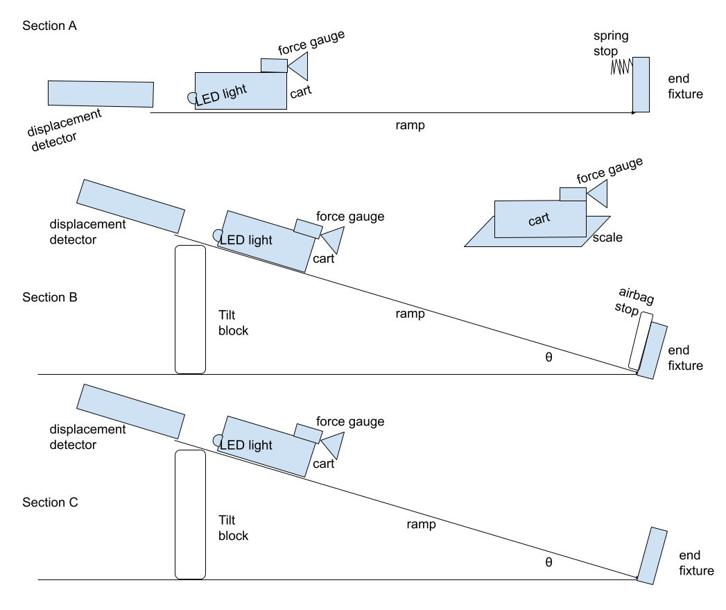
Describe the experiment
Start by opening the computer data acquisition program, in the Connection window, click WDSS button , then check both the displacement data link and force gauge data link options to pair up the computer with the instruments. The pairing name is “Bournolli80” in this experiment.
The cart’s LED light and force gauge are turned on with separate switches in the assembly. The displacement detector relies on the cart LED light. The force gauge uses a momentary switch button to initiate the wireless pairing.
The wireless pairing is interrupted several times during the 3 sections of the experiment. To re-establish the connection, press the force gauge’s momentary switch button once and click “Yes” to reestablish the wireless link in the computer data acquisition program.
The Google Sheet Table 1 for Section A has this format,
When the velocity window pane acquires velocity curve, the Vi bracket point is set to the starting of the bending of the curve from horizontal, and Vf bracket point is set to immediately adjacent to the complete rebending of the curve to horizontal.
In the force window pane, the start-stop brackets are manually dragged to as close to the same range as the velocity curve’s bracket range.
For Section B,
The Google Sheet Table 2 for this section has this format,
Three configurations of the short distance were tried, 40cm, 30cm, and 60cm. It was found that, at 40cm and 30cm, the airbag is powerful enough to produce cart oscillation at the end of the collision course. And 60cm or above can deflate the airbag without obvious oscillation at the end of the collision course. So, the short distance (for small Vi) is set to 60cm, and the long-distance (for large Vi) is set to 100cm.
For Section C,
The Google Sheet Table 1 for Section C has this format,
The maximum force that the force gauge can record is about 55N, and when the ramp is firmly pressed onto the workbench, the maximum force during the collision without airbag is greater than 55N and not recorded. So, the ramp can shift during the impact to reduce the measured force to within recordable range.
After all data is recorded, turn off the cart’s LED light switch, and it also turns off the electronic force gauge.
Results and Analysis
The first section of the experiment result is pictured in the following Picture 1 for the first data entry.
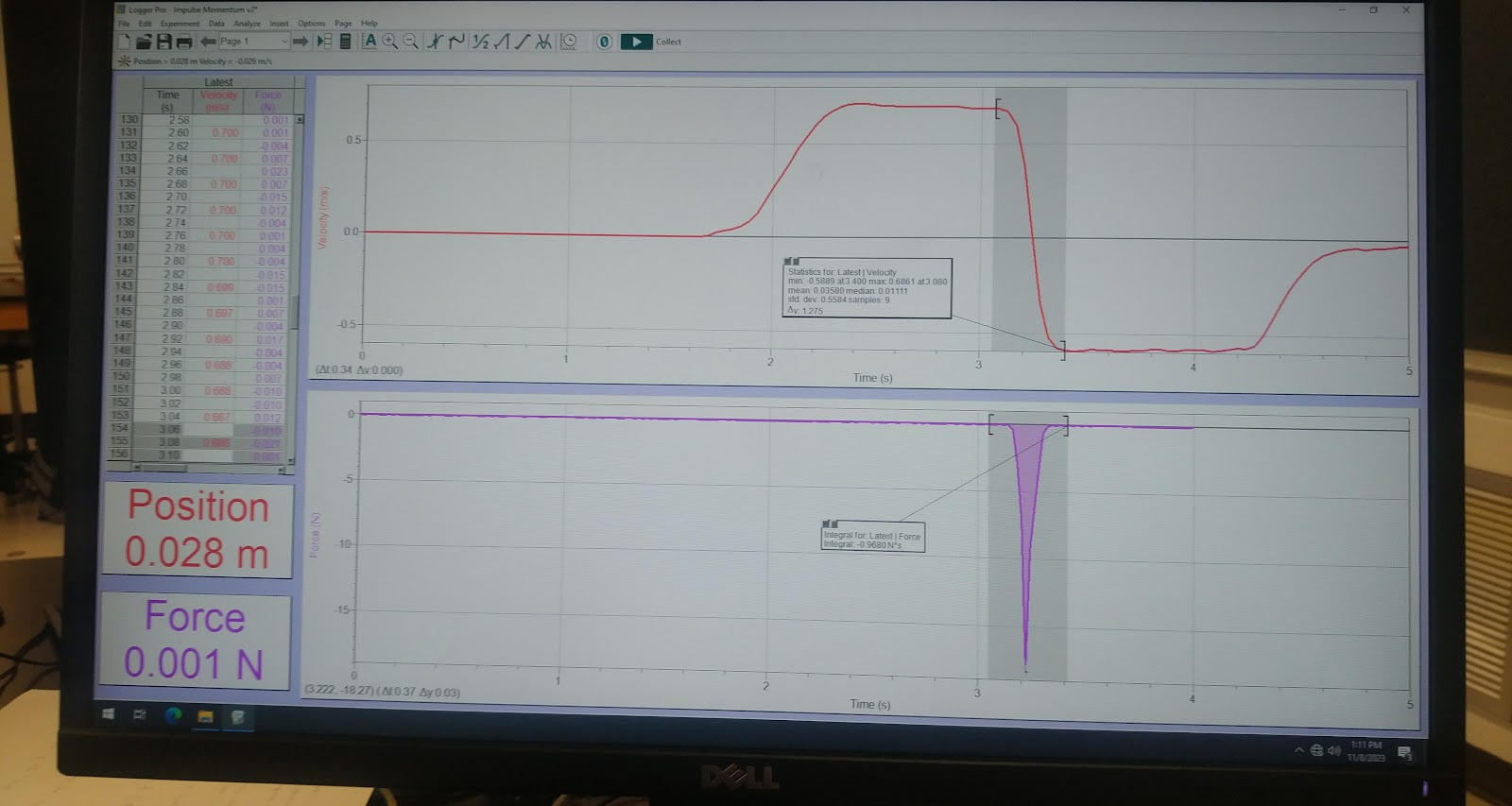
Picture 1.
The first section of this experiment’s result are shown in the following Table 1.
Table 1.
Sample calculation for the first row, Δp = mvf-mvi = 0.7730*(-0.5889)-0.7730*(0.6861)=-0.985575=-0.9856
; % difference = ((-0.9856)-(-0.9689))/(((-0.9689)+(-0.9856))/2)*100=1.71 .
The second section of the experiment result is pictured in the following Picture 2 for the first data entry.
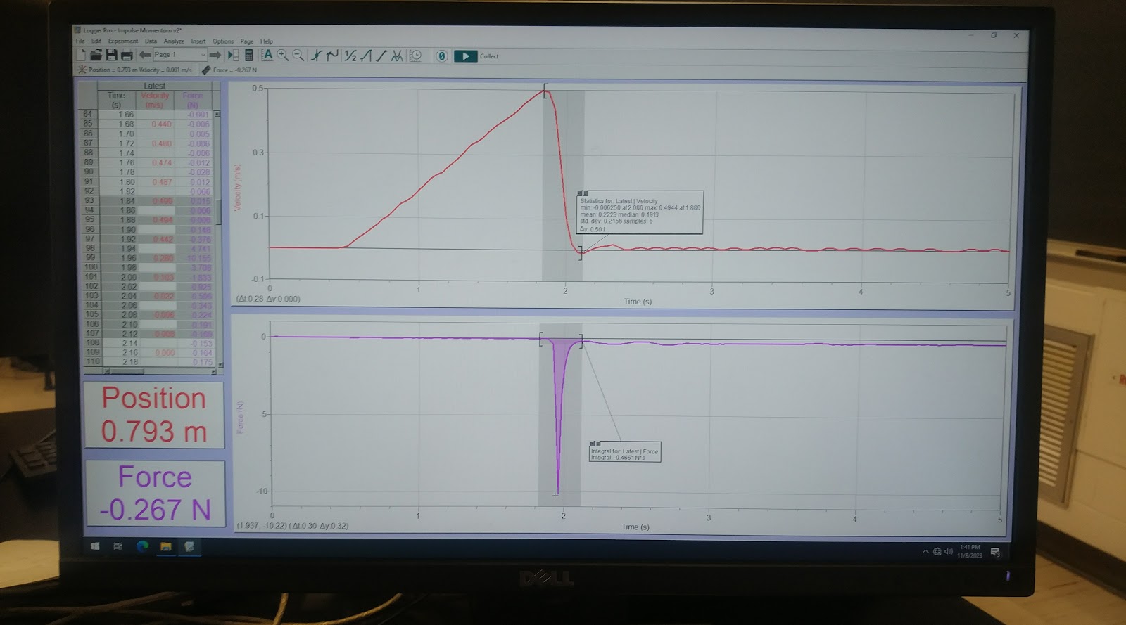
Picture 2.
The second section of this experiment’s result is shown in the following Table 2.
Table 2.
Sample calculation for the first row, Δp = mvf-mvi = 0.7730*(-0.00625)-0.7730*(0.4944)=-0.3870
; % difference = ((-0.3870)-(-0.4651))/(((-0.3870)+(-0.4651))/2)*100=-18.33 .
The third section of the experiment’s result is in the following Picture 3 for the 5th data entry.
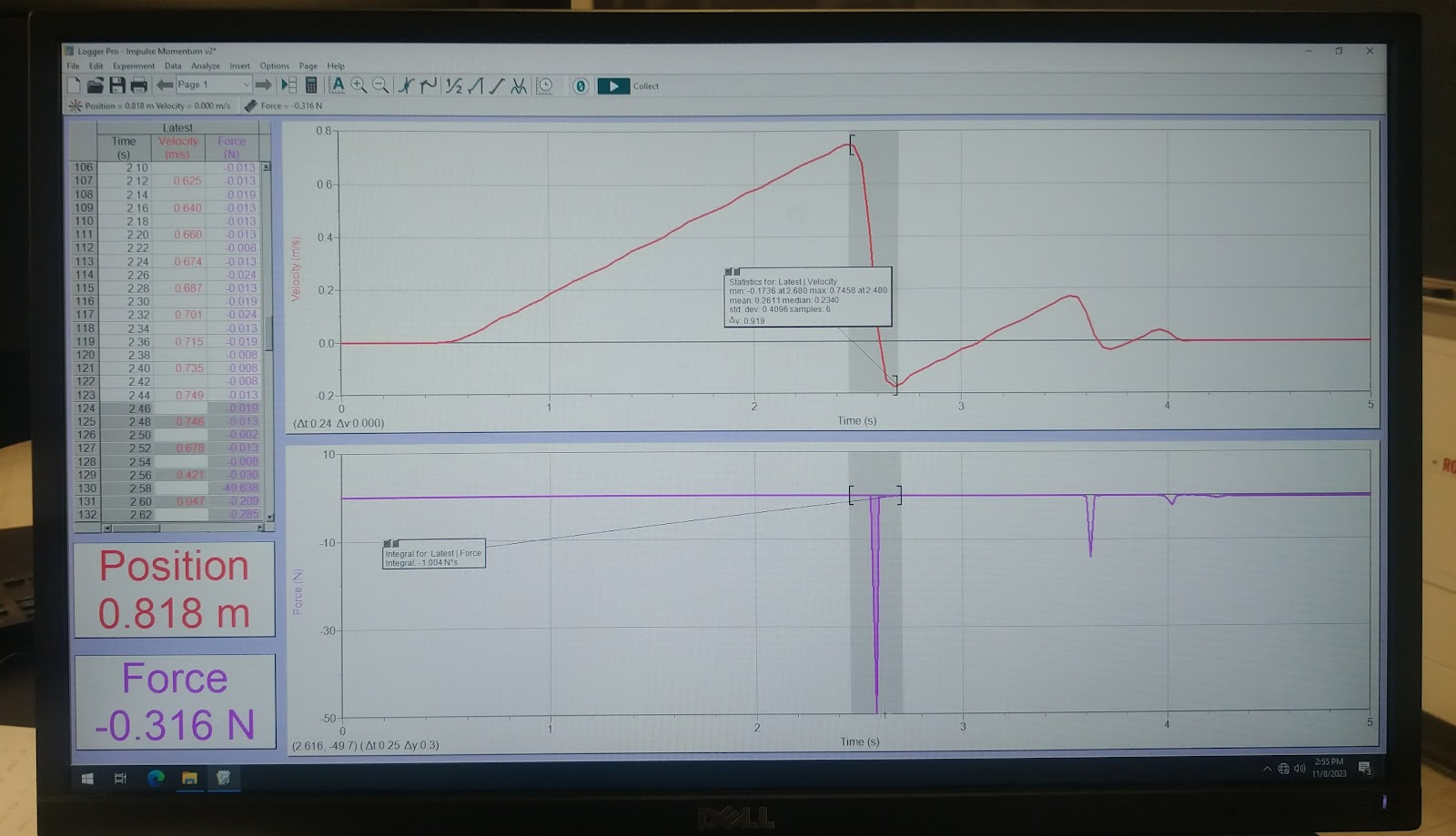
Picture 3.
The third section of this experiment’s result is shown in the following Table 3.
Table 3
Sample calculation for the 5th row, Δp = mvf-mvi = 0.7730*(-0.17360)-0.7730*(0.7458)=-0.7107
; % difference = ((-0.7107)-(-1.004))/(((-0.7107)+(-1.004))/2)*100=-34.21 .
Analysis
Section A Table 1’s Δp values are between -0.9Ns and -1.0Ns and J=FΔt values between -0.88Ns and -1.0Ns. The maximum forces of the collisions are between 10N and 21N. For each of the 3 entries, the %difference is between 1.71% and 3.17%. So, the integration result impulse J is very close to the measured momentum change.
The characteristics of Vi (m/s) versus Max force (N) for section A of this experiment are shown in below Graph 1.
Graph 1.
The higher the initial velocity, the higher the magnitude (absolute value) of maximum force.

This is reasonable because a spring’s force is Fspring = -x*k , where k is the spring constant.
The higher the initial velocity, the higher the collision impulse. And the higher the maximum force indeed produces larger integration over time.
The higher the Fspring, the higher displacement x of spring compression also means a longer collision time course, which means increased force integration over time.
Section B Table 2’s Δp values are between -0.38Ns and -0.56Ns and J=FΔt values between -0.46Ns and -0.67Ns. The maximum forces of the collisions are between 9.8N and 10.2N for the low initial Vi and between 11.8N and 13.8N for the high initial Vi. For each of the 6 entries, the %difference is between 9% and 18%. So, the integration result impulse J is also close to the measured momentum change.
The characteristics of Vi (m/s) versus Max force (N) for section A of this experiment are shown in below Graph 2.
Graph 2.

Similar to Graph 1. The higher the initial velocity, the higher the magnitude (absolute value) of maximum force.
Same principle as Graph 1, A spring’s force is Fspring = -x*k , where k is the spring constant.
The higher the initial velocity, the higher the collision impulse. And the higher the maximum force indeed produces larger integration over time.
The higher the Fspring, the higher displacement x of spring compression also means a longer collision time course, which means increased force integration over time

Furthermore, the 3 low initial Vi, created with the short release distance of 60cm, all have smaller (absolute) maximum force than the 3 high initial Vi, created with the short release distance of 100cm
As shown in Table 2, the 3 low initial Vi (about 0.5m/s) runs have an average of -10.31N maximum force.
Also, as shown in Table 2, the 3 high initial Vi (about 0.73m/s) runs have an average of -13.20N maximum force.
Section C Table 3’s Δp values are between -0.48Ns and -0.71Ns and J=FΔt values between -0.59Ns and -1.1Ns. The maximum forces of the collisions are between 9.8N and 10.2N for the low initial Vi and between 11.8N and 13.8N for the high initial Vi. For each of the 6 entries, the %difference is between 19% and 58% . So, the integration result impulse J deviates from the measured delta momentum is quite large.
The characteristics of Vi (m/s) versus Max force (N) for section A of this experiment are shown in below Graph 3.
Graph 3.

Contrast to section B’s Graph 2 and Table 2. The maximum force magnitudes without an airbag are much higher (average 36.5N and 53.5N for low and high Vi respectively) than with an airbag (average 10.3N and 13.2N for low and high Vi respectively) even though the initial velocity Vi are similar between section B’s runs and Section C’s runs.
The difference between maximum forces is about 36.5N/10.3N=~360% and 53.5N/13.2N=~405%.
As shown in Table 3, the 3 low initial Vi released runs have an initial velocity of about 0.52m/s, and high initial Vi released runs have an initial velocity of about 0.75m/s. These are very close to Table 2’s initial Vi velocities.
Also, comparable impulse Js are recorded in Table 2 and Table 3 for the runs with and without an airbag:
for low Vi, the impulses Js are about -0.5Ns with an airbag and -0.7Ns without an airbag;
for high Vi, the impulses Js are about -0.6Ns with an airbag and -0.1Ns without an airbag.
Discussion
Compared to theory
Section A Table 1’s theoretical integrated impulse J is within 3.2% difference from the measured momentum change in Table 1. This means that all the forces acting on the cart object are measured properly, and velocity and displacements are measured without problem. This is likely attributed to the small forces involved that don’t make the ramp apparatus shift and move during a collision.
Section B Table 2’s theoretical integrated impulse J is within 18% difference from the measured momentum change in Table 2. This is likely also attributed to the small forces involved that don’t make the ramp apparatus shift and move during a collision.
Section C Table 3’s theoretical integrated impulse J has a 19% to 58% difference from the measured momentum change in Table 2. This is likely attributed to the large forces that can make the ramp apparatus shift and move during velocity and force data collection.
Compare collision between with and without an airbag
Contrast between section B’s Graph 2 and Table 2 and section C’s Graph 3 and Table 3 are expected. The maximum force magnitudes without an airbag are much higher than with an airbag even though the initial velocity Vi are similar because the airbag extends the collision time course, as seen between Picture 2 and Picture 3.
Without an airbag, Picture 3 shows a steeper velocity slope and shooter time course. According to
titfFnetdt=mvf-mvi= -mvi , when Vf is zero
, when the time interval between ti and tf, the force will need to be larger to obtain the same momentum change.
Compare the Δp between Section B’s Graph 2 and Table 2 and Section C’s Graph 3 and Table 3; the momentum changes during a collision are very similar with and without an airbag, are expected. This is because momentum change only concerns about (mvf-mvi)=-mvi , when the objection is stopped at the end of the collection when Vf is zero. We use the ramp incline length to align the vi initial velocity between section B and section C of the experiment.
This means that, just by extending the collision time course time interval, the maximum force on the object can be reduced. In this experiment, the force reduction is between 360% and 405%, as shown in Analysis section C.
Uncertainty
The weighing scale has an uncertainty of 0.0001kg (0.1g). This affects both the bob mass and the hanging force.
Friction is not measured by the force gaugue even though friction between cart and ramp can contribute to cart velocity change.
The velocity has a computer electronic uncertainty of 0.001 m/s. The maximum force has an uncertainty of 0.1N.
The ruler for the ramp has a graduation of 1mm. So, the uncertainty of slope length is 0.001m.
Difficulties
The large % difference in section C is due to the unattached force gauge after the cart bounces back from impacting the ramp’s stop fixture. As depicted in the following picture 4, annotated from Picture 3.
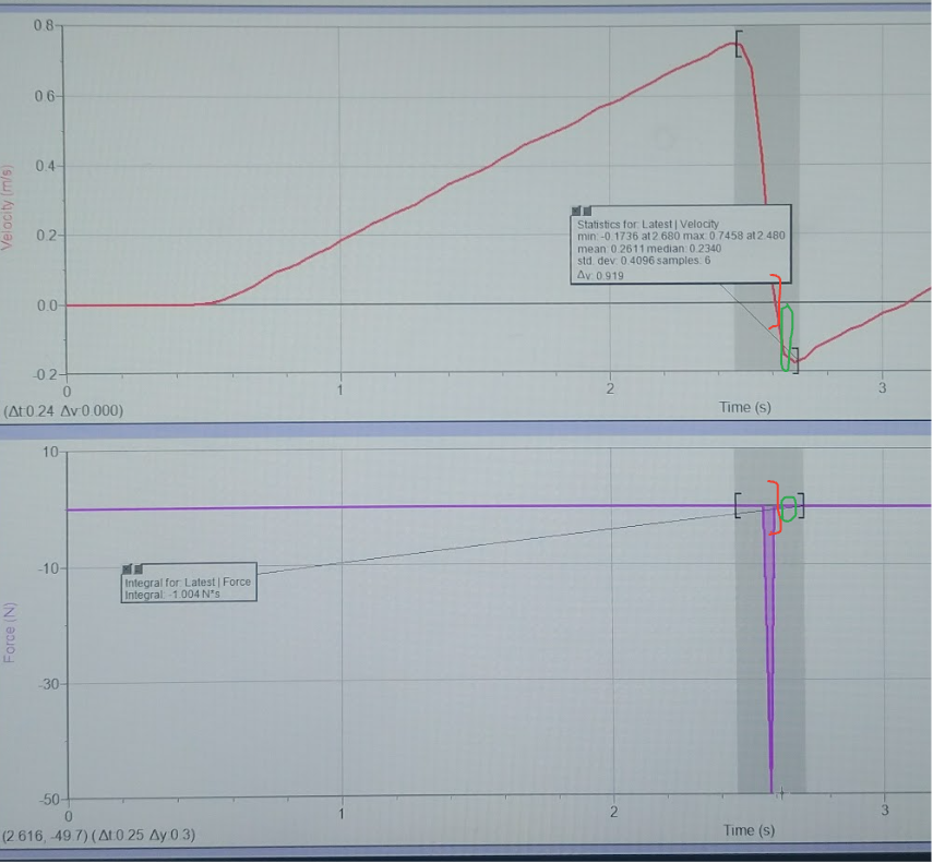
Picture 4.
The green circles mark the time when velocity is still changing rapidly, but the force gauge is not attached to anything because the cart bounces back, so force gauge integration is not correlated to the velocity plot during the green circled short time period. For an accurate calculation, velocity should only change when some force is measured because the derivation,
titfFnetdt=titfmadt=titf(mdv/dt)dt
, relies on acceleration and Fnet to correlate to velocity, and when F suddenly is not measured(for example, the entire measuring ramp bumped forward and force gauge is no pressed against anything), there will be difference between the integration and velocity change.
This problem is not present in Picture 1 and Picture 2, which have small forces measured when the velocity changing rates are smooth and small at the beginning and near the end of the impact time period.
Conclusion
My experimental measured data points in Table 1 through Table 3 show a % difference at reasonably low ranges, lower than 19%, except Table 3. And the trend of reduced maximum force with airbags has expected characteristics.
Restatement of the objection of this experiment is to measure impulse by velocity change and integral of force over the collision time course to corroborate the measurement with maximum force acting on an object. The maximum force measured indeed corroborates with the theory of integral of force, and the reduced maximum force via extended collision time course interval is demonstrated between section B and section C experiments with and without an airbag. The experiment is overall a success.
Questions
1. Compare and contrast the results from collisions with the light spring and those with the
airbag. What differences did you observe in terms of impulse and force? Explain the
possible reasons behind these differences.
With a light spring, the impulse is greater (almost twice as large) for the same initial velocity.
This is because the spring gives the cart a final momentum with a similar magnitude of velocity, just oppositive direction. In terms of impulse, for a spring,
impulse=mvf-mvi and vf and vi have similar magnitude , impulse -2mvi
; for an airbag,
impulse=mvf-mvi , and vf 0 , impulse -mvi
In terms of maximum force, airbag has smaller maximum force because the integration of force over time is smaller to reach only about half of the impulse as the spring’s impulse.
In terms of the force curve, with the light spring, force is at its largest when velocity is zero at the middle of the collision course; with an airbag, force is very close or equal to zero when velocity is zero at the end of the collision course.
This is because the spring stores potential energy when compressed.
Work = - Ep , when the spring resists the oncoming object and gets compressed backward, the spring does negative work and stores positive potential energy.
Force is at its largest when compressed to the maximum when the object is turning around to be expelled when velocity is zero because Fspring = -x * k.
An airbag does not store potential energy. When the airbag is flattened, there is no force to push the object.
2. Explain how the concept of impulse can be used to minimize injuries during a car crash.
What other safety measures are based on this principle?
Using the integral formula,
titfFnetdt=mvf-mvi= -mvi when Vf is zero at the end of collision
, extending the time interval between ti and tf allows force to be smaller while resulting in the same momentum change.
Without the airbag, the driver’s collision time course starts when his face touches the steering wheel or dashboard, and the time course stops when his head is bounced back or crushed nearly instantaneously by the steering wheel base or dashboard with great force.
The airbag starts the collision course when it inflates and reaches the face of the driver, and the collision course runs for a longer time until the face travels to nearly touching the base of the airbag unit. When the time interval is extended, force is reduced.
The second aspect of airbag protection is the dissipation of energy when the airbag does not store potential energy while most other materials have some capacity to store potential energy. When potential energy is eliminated, overall, there is less energy to harm the driver.
Seat belt also works by a similar formula, by extending the collision time course interval. The driver’s chest impacts the seatbelt and the time course starts immediately; when the shoulder and head of the driver move forward to the maximum extent, the travel distance of the head and shoulder receives the impulse over a time period longer than without the belt and impacting the dashboard and nearly instantaneously bounced back or crushed. The longer the time course interval, the smaller the maximum force.

3. Discuss the practical applications of the impulse-momentum theorem. How is this
theorem relevant in real-life scenarios, such as car safety or sports?
The application of the integration of the force curve can be wide-ranging. The force curve can be made to be wider and shallower to reduce maximum force. For example, the car hood can be designed in a way that exerts resistance sooner and crumbles fast during the collision.
In sports, the jogging shoe insert can also be tested to see if it is firm enough to give resistance during strides so that the force curve is wide and shallow.
No comments:
Post a Comment