Cover page
Student name: John C Gibson
Course number: PHYS.1410L , Section 811
Instructor name: Benjamin MacConnell
Date of experiment: Oct 25, 2023
Partner’s name: (No partner)
Title of experiment:
Circular Motion and Centripetal Force
Objective: Measure a rotational weight object’s centripetal forces and rotational angular velocities, then combine the measurements with weighted object mass and set rotational radiuses to calculate the theoretical values of the 4 variables to verify the validity of the measurements by their deviation from theoretical calculations. The deviations will be characterized to determine the causes of experimental errors.
Introduction
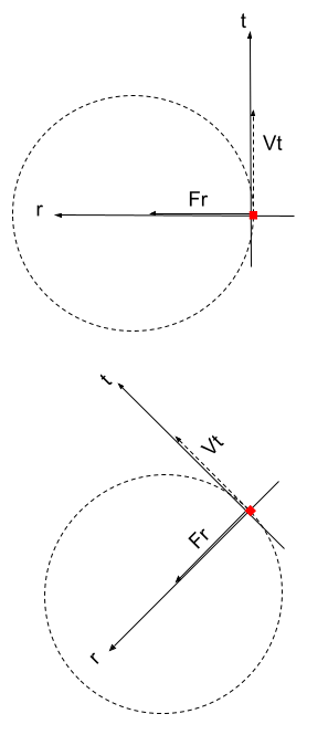
A rotating object with constant tangential speed requires a centripetal force to make the object change its velocity direction to create a circular motion, as shown in the diagram on the right. We choose the coordinate system with x-axis positive direction pointing to the center of the rotation circle and y-axis positive direction pointing to the same direction as the constant velocity Vt.
As the object moves along the circle, our coordinate system also rotates to keep the same coordinate directional scheme.
The centripetal acceleration is well-known as
a=v2/r=r2
, the centripetal force is
Fr=mr2 Equation 3.
.
There are 4 variables in the last equation. We will fix 2 variables of the last equation and measure the other changing variables in this experiment in the following 3 sections.
Fixed bob mass and rotational radius;
varying centripetal force and angular speed.
Fixed centripetal force and rotational radius;
varying bob mass and angular speed.
Fixed bob mass and centripetal force;
varying rotational radius and angular speed.
In all cases, the centripetal force is provided by a spring’s tension force that has been calibrated to gravitational force,
FM=Mg Equation 5.
Derivation:
To obtain the Fr, use Newton's second law,
Fr=mac
. Substitute ac with
ac=r2
, and we have
Fr=mr2
.
To obtain the rotation period T, recall that period is the time to complete a circle of 2pi angles.
T=2/
. Multiply both sides by and divide both sides by T,
=2/T
.
To obtain the percent difference between calculated centripetal force and measured force, we set it as so,
ABS F%=(Fmeasure - Fr)/Fmeasure100%
The absolute value will be used and referred to as “ABS” in calculations.
Without the absolute function,
F%=(Fmeasure - Fr)/Fmeasure100%
Steps
Start by opening the computer data acquisition program and checking whether the timing gate is functioning.
For section A (varying force)
Weigh the bob mass with 2 brass disks together with the center piece that will be the fixed mass in this section.
Enter the Force window and enter the fixed values of bob mass and fixed radius of 0.15m
Hook the bob mass to the vertical swing string and to the center spring’s string.
Hook a hanging mass of 0.065kg to the bob mass’s hook, and record this hanging weight in the data aquisition window.
Adjust the radius vertical bar to 0.15m. Adjust the spring’s fixture point so that the vertical swing string is vertical and aligned to the 0.15m distance.
Adjust the center indicator height so that the orange point of the spring is at the level of the indicator.
Remove the hanging mass.
Rotate the rotation apparatus so that the centripetal force causes the bob mass to settle to the 0.15m distance, which is indicated by the orange point of the center spring is at the level of the indicator.
Maintain the rotation as step 8, and click on START of the data aquisition window.
The timing will stop automatically after 10 revolutions. If no errors in entered data, click ACCEPT in the data acquisition window.
Repeat from this section’s step 4, for 5 additional trials, each time use a hanging mass of 0.055kg, 0.045kg, 0.035kg, 0.025kg, and 0.015kg.
For section B (varying bob mass)
Enter the Mass window and enter the fixed values of hanging mass force of 0.055kg and fixed radius of 0.15m.
Reassemble the bob mass with only the center piece. Weigh this new bob mass, and record this mass in the data aquisition window.
Hook the bob mass to the vertical swing string and to the center spring’s string.
Hook a hanging mass of 0.055kg to the bob mass’s hook.
Keep the radius vertical bar to 0.15m. Adjust the spring’s fixture point so that the vertical swing string is vertical and aligned to the 0.15m distance.
Adjust the center indicator height so that the orange point of the spring is at the level of the indicator.
Remove the hanging mass.
Rotate the rotation apparatus so that the centripetal force causes the bob mass to settle to the 0.15m distance, which is indicated by the orange point of the center spring is at the level of the indicator.
Maintain the rotation as step 8, and click on START of the data aquisition window.
The timing will stop automatically after 10 revolutions. If no errors in entered data, click ACCEPT in the data aquisition window.
Repeat from this section’s step 2, each time with an additional brass disk added to the bob mass assembly, 4 additional data entries with 1 additional brash disk, 2 additional brash disks, 3 additional brash disks, and 4 additional brash disk.
For section C (varying radius)
Enter the Radius window and enter the fixed values of hanging weight force of 0.055kg and bob mass the same as Section A’s bob mass.
Hook the bob mass to the vertical swing string and to the center spring’s string.
Hook a hanging mass of 0.055kg to the bob mass’s hook, and record this trial’s radius of 0.14m in the data aquisition window.
Adjust the radius vertical bar to 0.14m. Adjust the spring’s fixture point so that the vertical swing string is vertical and aligned to the 0.14m distance.
Adjust the center indicator height so that the orange point of the spring is at the level of the indicator.
Remove the hanging mass.
Rotate the rotation apparatus so that the centripetal force causes the bob mass to settle to the 0.14m distance, which is indicated by the orange point of the center spring is at the level of the indicator.
Maintain the rotation as step 8, and click on START of the data aquisition window.
The timing will stop automatically after 10 revolutions. If no errors in entered data, click ACCEPT in the data aquisition window.
Repeat from this section’s step 3 three times, but each time increase the trial’s radius by 0.01m, obtaining additional data for radius 0.15m, 0.16m, and 0.17m.
After the three experiment Sections are complete, enter Save in the data aquisition software. Then enter the recorded timing, mass, force, into Table 1 through 3 in Google Sheet. And then perform calculations for ω(rad/s), Fr=mrω^2 (N), ABS(ΔF(%)), and ΔF(%) inside Google Sheet.
Apparatus and Procedure
Complete list of equipment
Labeled block diagram of each part of the experiment
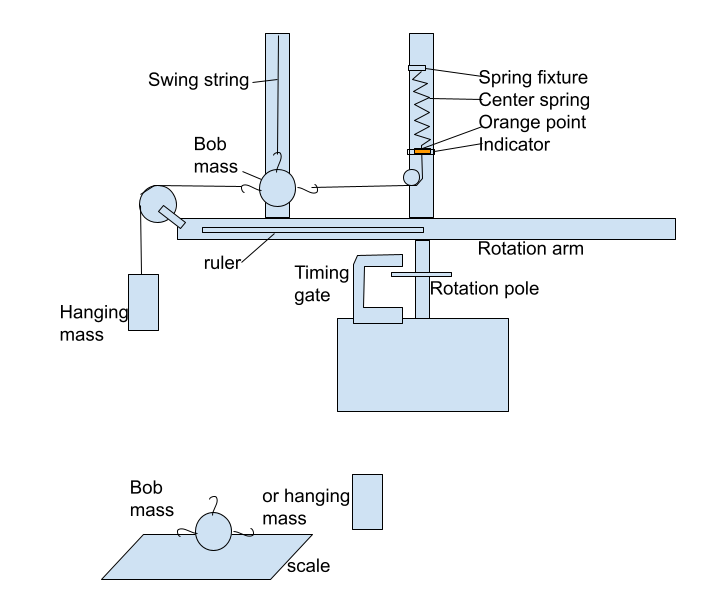
Describe the experiment
Start by opening the computer data acquisition program and checking whether the timing gate is functioning. This entails using the home page of the Circular Motion program’s Start button to test the timing gate with manual rotation of the rotation arm. The 3 sections of this experiment each has its own computer program window, titled Force, Mass, and Radius.
For Section A, don’t unhook the bob mass from the swing string once it is hooked in because we maintain the same bob mass in this Section A. Use the rotation pole to rotate the rotation arm, take care not to let finger interfere with timing gate because the electronic gate is a photo-sensitive device. For each trial, the computer data aquisition program stops when 10 revolution is reached. And the time for the 10 rotation is displayed.
The Google Sheet Table 1 for Section A has this format,
Enter the Period T by dividing the timing of 10 rotations by 10. Don’t use the computer-generated ω. We only use the computer program to obtain Period T.
The Google Sheet should be set up to calculate by =2/T .
Once one entry is obtained, stop the rotation and hook the hanging weight to the bob mass’s hook, 6 trials, with 0.065kg, 0.055kg, 0.045kg, 0.035kg, 0.025kg, 0.015kg, respectively.
In between changing the hanging mass, the spring fixture point needs to be adjusted, the higher the hanging mass, the higher the fixture point so to increase the spring’s tension to keep the bob’s static position at the constant 0.15m.
For Section B, do unhook the bob mass from the swing string between trials because the bob mass needs to be disassembled and reassembled with additional brass disk in this Section B. Also, this section uses 0.055kg hanging mass as a constant. And radius is constant 0.15m.
The Google Sheet Table 2 for this section has this format,
Enter the Period T by dividing the timing of 10 rotations by 10. Don’t use the computer-generated ω. We only use the computer program to obtain Period T.
The Google Sheet should be set up to calculate by =2/T .
Once one entry is obtained, stop the rotation and reassemble the bob mass, 5 trials, with no additional brass disks, 1 additional brass disk, 2 additional brass disks, 3 additional brass disks, and 5 additional brass disks, respectively.
In between changing the bob mass, the spring fixture point does not be readjustment because the hanging weight force is fixed, which matches the centripetal force.
For Section C, don’t unhook the bob mass from the swing string once it is hooked in because we maintain the same bob mass in this Section. The Google Sheet Table 1 for Section C has this format,
Enter the Period T by dividing the timing of 10 rotations by 10. Don’t use the computer-generated ω. We only use the computer program to obtain Period T.
The Google Sheet should be set up to calculate by =2/T .
Once one entry is obtained, stop the rotation and hook the hanging weight to the bob mass’s hook, 4 trials, with 0.14m, 0.15m, 0.16m, 0.17m radius, respectively.
When changing the radius for each trial, the spring fixture point needs to be readjusted, the wider the radius, the lower the fixture point so to reduced the spring tension and allow the bob’s rest static position to extend further.
Results and Analysis
The first section of the experiment’s timing result is pictured in the following Picture 1.
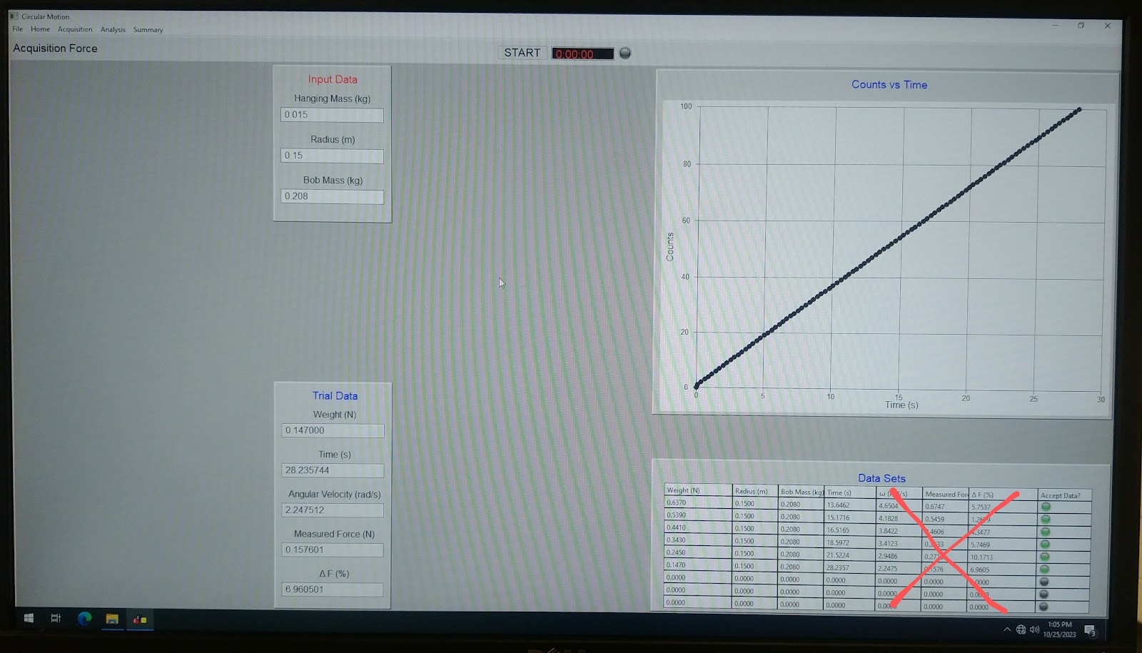
Picture 1.
Notice that we only use the Time of 10 rotations of the computerized data collection, the and Force discarded.
The first section of this experiment’s result calculated centripetal force, bob mass, hanging force, rotational radius, rotational angular period/speed, are shown in the following Table 1.
Table 1.
Sample calculation for the first row, Period T = Time 13.6462s / 10 = 1.36462(s); ω=2*3.14159/1.36462=4.6043; Fhang=0.065*9.8=0.637(N); Fr=mrw^2=0.2080*0.15*4.6043^2=0.6614 (N); ΔF(%)=(0.637-0.6614)/0.637*100%=-3.8%; ABSΔF(%)=|-3.8%|=3.8%
The trend line of deltaF% is shown in the following Graph 1.
Graph 1.

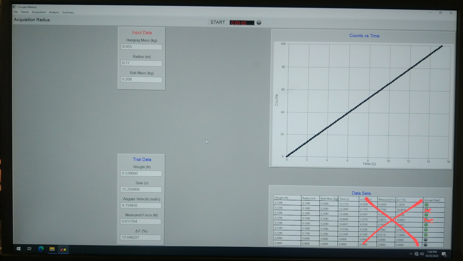
The second section of the experiment’s timing result is pictured in the following Picture 2.
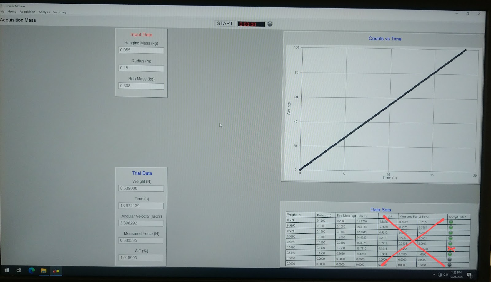
Picture 2. Data entries erroneously entered were crossed out with red.
Notice that we only use the Time of 10 rotations of the computerized data collection, the and Force discarded.
Also, the computer data acquisition has a redundant entry of Time 15.1716(s) that should be discarded.
The second section of this experiment’s result calculated centripetal force, bob mass, hanging force, rotational radius, rotational angular period/speed, are shown in the following Table 2.
Table 2.
Sample calculation for the first row, Period T = Time 10.8164s / 10 = 1.08164(s); ω=2*3.14159/1.08164=5.8089; Fhang=0.055*9.8=0.539(N); Fr=mrw^2=0.1080*0.15*5.8089^2=0.5466 (N); ΔF(%)=(0.539-0.5466)/0.539*100%=1.4%; ABSΔF(%) = |-1.4%|=1.4%
The trend line of deltaF% is shown in the following Graph 2.
Graph 2

The third section of the experiment’s timing result is pictured in the following Picture 3.
Picture 3. Data entries erroneously entered were crossed out with red.
Notice that we only use the Time of 10 rotations of the computerized data collection, the and Force discarded.
Also, the computer data acquisition has a redundant entry of Time 15.1716(s) that should be discarded.
The first section of this experiment’s result calculated centripetal force, bob mass, hanging force, rotational radius, rotational angular period/speed, are shown in the following Table 3.
Table 3
Sample calculation for the first row, Period T = Time 14.5860s / 10 = 1.45860(s); ω=2*3.14159/1.45860=4.3077; Fhang=0.055*9.8=0.539(N); Fr=mrw^2=0.2080*0.14*4.3077^2=0.5404 (N); ΔF(%)=(0.539-0.5404)/0.539*100%=-0.3%; ABSΔF(%)=|-0.3%|=0.3%
The trend line of deltaF% is shown in the following Graph 3.
Graph 3

Analysis
Section A Table 1’s Fr increases as ω increases because Fr=mr2 , and m and r are fixed. Fr and ω are directly proportional to each other.
The characteristics of ABS ΔF(%) of the first section A of this experiment is shown in the Graph 1.
Higher force, higher error ΔF(%)
*Lowering force, lower error ΔF(%)
Higher ω, lower error ΔF(%)
*Lower ω, higher error ΔF(%)
Force trend down and ω trend down cancel each other's effect on error ΔF(%);
However, force change by 4 folds and ω change by 2 folds, so force trend down error ΔF(%) dominates.
Section B Table 2’s ω decreases as bob mass m increase because Fr=mr2 , and Fr and r are fixed. ω and m are inversely proportional to each other.
The characteristics of ABS ΔF(%) of the second section B of this experiment is shown in the Graph 2.
*Higher mass, lower error ΔF(%)
Higher ω, lower errorΔF(%)
*Lower ω, higher error ΔF(%)
Mass trend and ω trend cancel each other. So, the trend line is nearly flat, with no increase or decrease.
Section C Table 3’s ω increases as radius r decrease because Fr=mr2 , and Fr and m are fixed. ω and r are inversely proportional to each other.
The characteristics of ABS ΔF(%) of the second section of this experiment can be shown in the Graph 3.
*Higher radius, higher error ΔF(%)
Higher ω, lower errorΔF(%)
*Lower ω, higher error ΔF(%)
Radius and ω trend enhance each other, so the ΔF(%) trend line goes up significantly as the radius increases.
Discussion
Compared to theory
Section A Table 1’s Fr increases as ω increases, however, there are more trials of Mg smaller than Fr, indicating
rotation speed is overrunning, and the orange point is often slightly below the indicator during rotation.
Section B Table 2’s ω decreases as bob mass m increase, however, there are more trials of Mg smaller than Fr, indicating rotation speed is overrunning, and the orange point is often slightly below the indicator during rotation.
Section C Table 3’s ω increases as radius r decrease, all tials have Mg smaller than Fr, indicating rotation speed is overrunning, and the orange point is likely often below the indicator during rotation.
ΔF(%) shows the difference between scale-weighed centripetal force and calculated Fr based on rotational ω .
This is the difference between the calculations of the 2 different equations,
Fr=mr2 Equation 3.
FM=Mg Equation 5.
When ΔF(%) is positive, it means the rotation speed is insufficient, and the orange point is likely slightly above the indicator.
When ΔF(%) is negative, it means the rotation speed is overrunning, and the orange point is likely slightly below the indicator.
In the result Table 1 and Table 2, both negative and positive ΔF(%) exist, which means that the manual reinvigorating the turning arm both over reinvigorating and under reinvigorating in different trials of the experiment. No particular trend of the ΔF(%) relating to Fr or radius or bob mass.
On the other hand, the ABS ΔF(%) has characteristics as shown in result analysis. The trend lines can be summarized as the following,
Higher force, higher ABS ΔF(%); lowering force, lower ABS ΔF(%).
Higher ω, lower ABS ΔF(%); lower ω, higher ABS ΔF(%).
Higher mass, lower ABS ΔF(%).
Higher radius, higher ABS ΔF(%).
These 4 points are expected because the higher the centripetal force, the more force to make the center spring oscillate and increase ABS ΔF(%). The higher the bob mass, the more inertia to stabilize/stop the spring’s oscillation so that the operator’s hand-eye coordination can narrow down the error ABS ΔF(%). And the higher radius, the lower the ω. Recall that the entire rotation arm has angular momentum too. And the lower the ω, the lower the angular momentum of the whole system, which makes the system more prone to change angular velocity by manual reinvigoration, and “change” is the very definition of Δ.
Uncertainty
The weighing scale has an uncertainty of 0.0001kg (0.1g). This affects both the bob mass and the hanging force.
Friction is not a direct uncertainty of the calculated force Fr because Fr is calculated based on timing period T and and bob mass. However, friction slows down the turning arm of the apparatus, which we manually reinvigorate the rotation. So, the uncertainty is hand-eye coordination to regenerate force to align the indicator with the orange spring point. This uncertainty is reflected in the T. But it is hard to put a number of decimal places to it. Friction is an indirect contributor to uncertainty.
The timing period has a computer electronic uncertainty of 0.0001 seconds per 10 rotations. So, the actual uncertainty of T is 0.0001/10=0.00001 seconds.
The ruler for the radius setup has a graduation of 1mm. So, the uncertainty of the radius is 0.001m.
Difficulties
The hand-eye coordination to regenerate force to align the indicator with the orange spring point is the biggest difficulty of this experiment. This fluctuation is reflected in the T and contributes to ΔF(%) the greatest.
Conclusion
My experimental measured data points in Graph 1 through Graph 3 show ΔF(%) at reasonably low ranges. And the trend of ABS ΔF(%) has reasonable characteristics.
Restatement of the objection of this experiment is to measure a rotational weight object’s centripetal forces and rotational angular velocities, then combine the measurements with weighted object mass and set rotational radiuses to calculate the theoretical values of the 4 variables to verify the validity of the measurements by their deviation from theoretical calculations. The deviation ABS ΔF(%) trend lines have been characterized in the analysis section and the logic behind the characteristics is understandable. The objection is achieved. My experiment was a success.
Questions
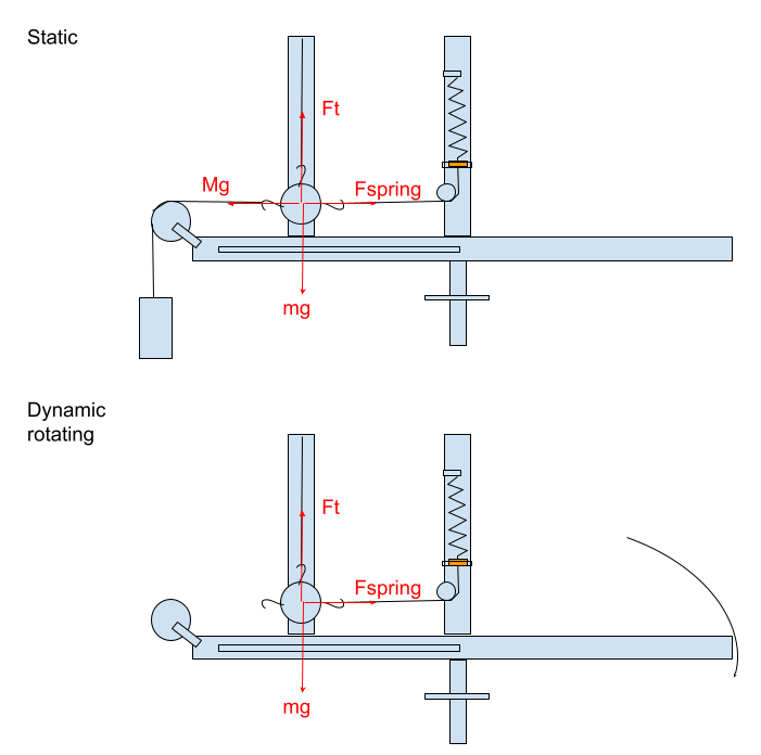
1.Draw free-body diagrams for the rotating mass in both static and dynamic scenarios.
2. When the radius is increased, does the period of rotation increase or decrease?
Fr=mr2
Radius is inversely proportional to . However, is inversely proportional to period. So, period is directly proportional to . So, period of rotation increases when radius is increased.
3. When the radius and the mass of the rotating object are held constant, does increasing
the period increase or decrease the centripetal force?
Fr centripetal force is directly proportional to . However, is inversely proportional to period. So, centripetal force decreases when period increases.
4. As the mass of the object is increased, does the centripetal force increase or decrease?
Centripetal force increases because it is directly proportional to m.
5. In the laboratory, did you observe any discrepancies between the centripetal forces
measured using Eq. 3 and Eq. 5? If so, what could be the reasons?
Fr=mr2 Equation 3.
FM=Mg Equation 5.
The biggest reason is that the spring’s orange point is manually controlled through the rotational pole during rotation. Assuming the orange point is perfectly aligned during the static phase,
if the orange point is above the indicator during rotation, it means that it rotates too slow, the centripetal force calculated Fr is lower than the calibrated Mg;
if the orange point is below the indicator during rotation, it means that it rotates too fast, the centripetal force calculated Fr is higher than the calibrated Mg.
The manual reinvigorating the rotation platform is not 100% accurate.
6. Could you discuss the significance of using the weight of the calibration mass as an
indirect method to measure the centripetal force?
As shown in the force diagrams, the static calibration mass-produced force Mg has the same magnitude of force as Fspring when bob mass at the radius r point. The only difference between Mg and Fspring is direction.
During rotation, the bob mass is controlled to stay at the radius r, which means the same magnitude force Fspring is exerted by the spring because it is common knowledge that a spring exerts the same force when stretched to the same length. But, now, Fspring=Mg is the centripetal force that keeps the bob object rotate at radius r point, as shown in the dynamic phase force diagram.
So, as long as the orange indicator is aligned with indicator both in static and dynamic phase, Fr=Fspring=Mg.

No comments:
Post a Comment