All prototype parts have their weights on the 250-gram-limit weighing chapter page. The entire series of this topic has 8 blogs:
Converged AIoT Developer Kit | Build Notes | Operating Notes | Ground Station Setup | Near The Edge Of Space | Endurance | Weight 250 Grams Breakdown | Build and Operation Substitutes
Frame Prototype Substitute

The prototype substitute frame in place of the production AIoT kit increases overall weight by less than 3 grams. This fuselage can be 24.3 grams at most after trimming with bearings 1 gram, in place of side walls 8.7 + tailblock 5 + battery tray 2.3 + bottom 2.4 with bearing blocks 6.8 grams. Swash 4.5 grams in place of 2.5 grams of production build. Linkage pushrod 2.2 + DFC link 0.3 + DFC pin s1.2 grams in place of linkage rod 0.8 + DFC link 0.9 + DFC pins 0.8 grams. This prototype substitute reduces 6 zip ties about 0.6 grams, reduces tail-bore insert of 0.7 grams, avoids a GPS tray of 0.5, omits motor stopper of 0.1 grams, and reduces 10 nylon washers and 2 steel washers of 0.6 grams. But this substitute incurs struts about 0.6 grams plus 0.7 grams extra bolting . Weight gain equation is
24.3+1+4.5+2.2+0.3+1.2-0.6-0.7-0.5-0.1-0.6+0.6+0.7-(8.7+5+2.3+2.4+6.8+2.5+0.8+0.9+0.8)=+2.1
. This weight gain can be shed with a lighter prototype motors by 1.1+0.3 grams, glued tail propeller by 0.3 grams,
However, cost-wise, the prototype saves 82 USD, without the production bearing block, sidewalls, and tail block at combined 81.97 USD. The parts cost saving equation corresponding to the weight equation is
10.49+2.20+8.67+5.24+5.99+5.19-0.12-0.00+0.00+0.00-(39.98+14.99+5.00+4+26.99+11.99+9.99+4.99+1.80)= -82.07
Cutting the thick rear corner needs the middle-speed setting on the rotary tool with a cutting disc, which often splatters hot plastic lava. To ease the work, the middle speed should be only used halfway from the rear on the sides, and the middle lower speed to just score the rest of the cut, and then use pliers to tear the plastic, as in the following picture. Cutting out the rear pedestal on 230 V2 saves 0.5 grams.

Cutting the enforcement extension plate needs the cutter disk axis to be mounted with spacing as in the picture here to allow clearance between the bay and the rotary tool chuck nut.  |  The cutting needs the rotary tool shaft sinking into the hollow part of the electronics bay plate. Cutting out side enforcement and electronics plate extension saves another 0.6 grams. |
 Cutting out the front lateral studs, saving 0.3 grams, for installing thicker battery packs is a mistake because thinner battery cells are available even for capacities higher than 900mAh. Reinforcing the seamline with bots and plates would add more weight than the original stud and screw weight.
Carving the shaft cage sides saves another 0.7 grams. The carving avoids wall studs along the pencil marking before carving. The carving should reserve 2-3mm edges from the straight stud walls. But first, the studs for the original canopy peg need to be drilled out with a 5mm drill bit. It can be done manually without an electrical drill with a chuck holder, as pictured below.
 Carving the shaft cage front needs a small diameter cutting disk, as in the following picture. The small diameter is obtained after a disk is worn out or trimmed. Carving the middle panel and shaft cage front saves another 0.7 grams.


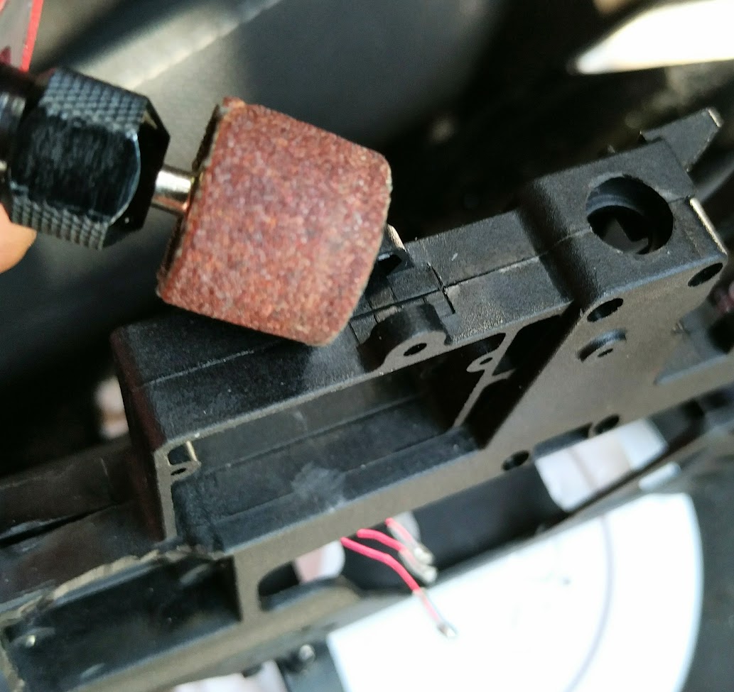
Cutting the bottom panel extensions saves another 0.3 grams. The bottom plate has a sharp join that is often the very first fracture the build encounters with a crash. The sharp join can be smoothed with the rotary sanding drum as the lower example. However, such an extra step doesn't improve the crash-breaking characteristics. The broken joint is repaired with a scrap patch from carving the main frame.

Cutting the front servo mount extension and rear servo cage enforcement double saves another 0.3 grams.


Cutting out the lips of the lower shaft bearing holder and final cleaning saves another 0.2 grams, including caving a dent in the vent window.
The final weight after all trimming is 21.6g, including the erroneous cutting out of the front lateral studs that reduced by 0.3 grams, as shown on the weight breakdown page.
Rail guard with this frame:
Kydex material is flexible and can be cut with household scissors. In the base build, we outlined the edge of the carving about 2-3mm from the straight stud wall. Here we drill 1.2mm anchor holes for the rail guard as close to the stud wall as possible or as far away from the plane edges as possible to maximize the strength of the anchor holes against tearing forces. Then the rail is attached by Kevlar threads or M1.5 screws.


Battery mount with this substitute frame:
Drill 3 holes flush and parallel to the ceiling of the front battery bay through the ceiling stud using a 1.5mm drill bit. The ceiling holes are 15mm from the edge.


The 2 holes on the right side of the craft (from the craft's perspective) should be closer to each other, shifting the middle hole from the center by about 5mm to avoid drilling beneath the seamline that would weaken the fuselage's strength. Then the zip ties need their corresponding holes through the ceiling to thread through as pictured above on the right.
Custom servo bracket with substitute fuselage: The vertical servo configuration is the shared knowledge and industry trend for giving rigidity of swashplate control. The 230s frame's front servo is already vertical, so, the front servo doesn't need a custom bracket. For the rear servos, we align the rear side of the servos to the axis of the rear fixture hole, as pictured below on the left, so that the servos can not be twisted and depressed into the servo cage by the screw standoff stopper. The upper strut, coincidentally, needs to be placed onto the corner of the anti-rotation bracket base, as pictured below on the right. For the rear servos, we have 2 options to make the custom bracket; below on the right, blade 230's landing skid set is used for struts, which have the same diameter as the Plastruct MS-160 Square Rod.


The screwdriver to install and service the upper custom rod needs to be inserted from the bottom of the craft through the middle plate. So, a conduit is drilled on the middle plate beneath the custom rod.


Wiha Philips #1 screwdriver or another driver with 3.5 inch shaft or longer is used to penetrate the conduit. The conduit to allow the long screw driver is about 5mm in diameter. Before any drilling, pre-treatment to smooth the injection seam line bump is needed to prevent slip.


Wiha Philips #1 screwdriver or another driver with 3.5 inch shaft or longer is used to penetrate the conduit. The conduit to allow the long screw driver is about 5mm in diameter. Before any drilling, pre-treatment to smooth the injection seam line bump is needed to prevent slip.

The drill bit for the holes on the craft is 1.4mm as seen in picture below on the right, and the drilling can be done using a chuck to pinch and twist the drill bit.


The boreholes on the bracket rods themselves should also be 1.4mm to prevent material warping with high pressure. The struts should be drilled from both end surfaces progressively to the center in the material. Drilling from one surface through often results in mis-aligned servos, which are hard to gauge the play. Before final assembly, the screws need to be filed of their protrusion because the splinters of the lower bracket prevents a snug fitting of servos. For the Blade 230 main frame, file and carve the upper strut 1mm along the contact surface with the cage roof wall. The final assembly uses the same Phillips #1 screw driver to fasten the bottom custom rod from underneath the craft. Then use M1.7 screw, or the landing skid's fastener screw, as the stopper to prevent the servo from sinking into the servo cage. The servos are fastened without washers to allow self-centering by the tapered screw heads. The M1.5 fasteners on the servo tabs need to be tightened evenly and progressively, checking the play in the process by shifting the servos up and down and probing for a snug fit.
Torque of this prototype setup is all the same as production build except "M1.5 self-centering screws for servo tabs. Torque to stop slop but not harder".
 The nylon landing skid rod option weighs exactly the same as ABS struts, which should not be a surprise because the density of ABS is known to be lighter than nylon, and the nylon part is smaller, more compact in volume.

In the upper right corner of the picture above, you can see that the gap for the anti-rotation zip-tie to thread through is very narrow. So, the zip tie must be pre-bent and pre-twisted, as pictured on the right, to fit the narrow gap.
The main frame kit comes with 2 different sizes of screw sets, Philips #1 and #0. If you receive the Philips #1 hardware, the screwdriver needed to fasten the main shaft cage is a 2mm slot driver instead of the official Philips #1 because Philips #1 screwdrivers with 1/8 inch shaft to go into the small bore holes is very rare in the market.
 The generic zip ties of 3mm width, such as the DWF branded product, can not replace the HyperTough 3mm wide zip tie even though they have the same nominal tensile strength of 18 lb. The generic zip tie simply breaks with a jerk of torque after the rotor spool-up and collective pitch suddenly change from negative to zero to positive, and the tail motor takes on countering the motor torque, all happening within a split of a second.
A set of servo links includes 1 long steel rod and 2 short steel rods. The long rod, after cutting out the center, non-threaded area, has 2 short segments, each for 1 rear servo link. One of the original short rod is used for a DFC link. The second short link, unmodified is used as the front servo link. The extra ball socket pair from a second purchase of servo link set has 1 rod for another DFC link. The extra ball socket pair from the second purchase has 2 ball sockets for the 2 DFC links.
 The short rods are still too long for the DFC link and need trimming out 2mm with the rotary cutting wheel. Once trimmed, the DFC link and the ball socket join tightly, giving a uniform length. Before installing the DFC swash control rods, the original Blade 180CFX hub has 2 swash-driving arms that must be removed to make way for DFC links. It was discovered that this prototype assembly had very robust resilience for crashes, and this assembly's DFC link length, as shown in the picture on the right, is replicated in the production DFC link. So, the production rotor's articulation range characteristics are identical to the prototype's.


 The generic zip ties of 3mm width, such as the DWF branded product, can not replace the HyperTough 3mm wide zip tie even though they have the same nominal tensile strength of 18 lb. The generic zip tie simply breaks with a jerk of torque after the rotor spool-up and collective pitch suddenly change from negative to zero to positive, and the tail motor takes on countering the motor torque, all happening within a split of a second.
A set of servo links includes 1 long steel rod and 2 short steel rods. The long rod, after cutting out the center, non-threaded area, has 2 short segments, each for 1 rear servo link. One of the original short rod is used for a DFC link. The second short link, unmodified is used as the front servo link. The extra ball socket pair from a second purchase of servo link set has 1 rod for another DFC link. The extra ball socket pair from the second purchase has 2 ball sockets for the 2 DFC links.

 The short rods are still too long for the DFC link and need trimming out 2mm with the rotary cutting wheel. Once trimmed, the DFC link and the ball socket join tightly, giving a uniform length. Before installing the DFC swash control rods, the original Blade 180CFX hub has 2 swash-driving arms that must be removed to make way for DFC links. It was discovered that this prototype assembly had very robust resilience for crashes, and this assembly's DFC link length, as shown in the picture on the right, is replicated in the production DFC link. So, the production rotor's articulation range characteristics are identical to the prototype's.


h The video on the right shows the F411 startup throttle reset to the lowest level, and servos travel down about 4.2mm=12mm*sin(83.0/4) to only a few millimeters above the base. This problem is unique to F411 software. It can not be fixed with the latest version, 4.2.11. Compared to substitute hardware, the software version 4.2.0 through 4.2.5 don't have the twitch in the other hardware. For this reason, our build uses Microheli Blade 230 shaft collar that is thin enough to avoid colliding with the swash.
The ESC setup for this prototype substitute is pictured on the right. The XT30 connector needs a half cut in between the poles for Kevlar string to tie it to the main frame, as pictured below.


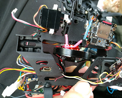
The overall build of prototype components:


Light-Weight BSR Frame For Fuel Economy
E-Flight BSR main frame is 23.2 grams and nominally saves 1.1 grams from the 230s frame. The following first 2 photos are of the same frame. Cleaning the frame reducing 0.6 grams (without erroneous trimming of the front battery bay stud) maximum should result in between 20.8g and 22.0g. The hardware screws weigh 1.1x10/9=1.2 grams. So the installation is between 20.8 +1.2=22g and 22+1.2=23.2g , worst case 23.2 grams.


When closing the main shaft cage, the screws go in from the left side of the craft(from the craft's first-person perspective) on the BSR main frame.
However, the E-Flight BSR anti-rotation bracket is 0.4 grams heavier than 230s' at 0.9 grams. So, the actual weight saving is 0.7 grams when the BSR frame is not further trimmed to save weight. One screw is not used because we use custom M1.7 long screws.


To compare the rear servo geometries, as shown in the picture above on the left, the servo fixture system is forward 1.2mm on the 230s frame. So, the BSR frame's servo setup has a more slanted servo rod toward swash. This can not be improved because we need to prevent servos from caving into the servo cage with a BSR frame, so we can't move the rear left servo forward 1.2mm, related to the cage geometry.
The servo tab location is marked in the picture above on the right and is 10mm behind the BSR frame's servo cage's upper front wall surface, as measured in the pictures below on the left. The placement of the 1.25mm bore holes is 10mm+2mm=12mm behind the upper front wall surface because the struts have a 4mm diameter and a 2mm radius. The counterpart of the 1.25mm half holes on the bottom plate is 12mm+1.4mm=13.4mm behind the lower front wall surface, as indicated in the picture below. The 1.4mm shift is due to the thickness of 4mm of the upper wall. The fixture hole diameter is 1.2mm. The extra thickness from the edge of the fixture hole to the wall's surface is (4mm-1.2mm)/2=1.4mm. The lower Wall's thickness is the same as the fixture hole diameter. The lower wall's surface is tangent to the fixture hole's edge, hence no extra thickness.


The servo fixture hole geometry, namely the width/height/depth of the BSR frames, is congruent to that of the 230s frames. The mentioned 13.4mm distance of the BSR frame is equivalent to having 14.6mm on the 230 frame from the wall to the fastener holes. This distance has a 14.6-13.4=1.2mm reduction in the BSR frame because the 230s frame moves the wall forward 1.2mm, which is the diameter of the servo fastener hole's diameter. In the 230 frame, the wall's inner surface is tangent to the hole; in the BSR frame, the wall is aligned to the hole axis. In either case of BSR or 230s, the axis-to-axis distance between the original fixture hole and the hole for custom struts is 14mm. The math is 13.4+0.6=14=14.6-0.6.

In the diagram here for the depth dimensions, the curious number 1.25mm of the fixture holes on the anti-rotation bracket are actually half-moon dents of 1.25 mm depth because the screw we use is 1.5mm in diameter, and the bracket's width is 6mm. So, the center of the 2 half moons is 0.5mm from the bracket's side edges. 0.5mm+(1.5mm/2)=0.5mm+0.75mm=1.25mm .
The 230s swashplate fits the 230s main frame unmodified. For the BSR frame, we need to trim the anti-rotation bar, first grind the top to form a flat surface. Use the cutting disk/wheel with the slowest rotary tool speed for this job. Then slice the 2 sides 45 degrees from the top to form a rough final shape.


Once the rough final shape is formed, draw a mental line vertical from the upper left corner down. The plastic material on the left side of the line needs to be preserved. Grind out the lower-right corner material to finalize the trim.


After the trimming, shorten the bar so it can escape the anti-rotation bracket in the event of a crash.
Unlike the 230s frame, the upper strut for the BSR frame should not be carved to prevent material warping. Instead, for the BSR frame, the anti-rotation bracket's groove needs to be carved, and our custom bracket sits on the flat surface of the anti-rotation bracket, as shown in the picture below on the left. This is because the BSR frame's servo cage ceiling is 1mm lower than the 230 frame's.


As pictured above on the right, the BSR frame's middle vent window is 1.5mm higher than the 230 frame's. So, the aviation computer USB port doesn't need frame carving. The example in the picture needs only a slight scraping of the inner edge with a craft knife.
Prototype Frames With Carbon Fiber Main Motor Shaft
When using prototype Blade 230s or BSR frame with the prototype 19mm thickness motor: This doesn't mean that the rotor mast will be lowered by 3.5mm and risking tail strikes by the main rotor. Remember that, in the extreme robotics build, we had shaft intrusion with the titanium shaft by 2.3mm with the prototype fuselage. Here with the carbon fiber shaft, we push the protrusion up and flush to the motor bottom plate, and our rotor mast is only lowered by 3.5mm-2.3mm=1.2mm. So practically, there is no risk of a tail strike or noticeable change of mechanical dynamics.
Electronics Bay Option Aviation Computer
This is a substitute mounting for the aviation computer for the acrylic base plate of the production build. It can save 0.9 grams.
The bus plug edge is flush to the edge of the electronic bay floor. The clear mounting tapes are 12x7mm, with 4 pieces on the front and 1 piece on the array of pins. The 7mm-wide USB socket protrusion will be our guide to fit the aviation computer into a temporary soft jig. The soft jig is made with foam mounting squares, as pictured below. Also, in the inside picture of the jig, you can see that the electronic bay floor has only a 2mm strip overlapping on the front of the aviation computer board. So, the 4 pieces of clear mounting tapes need to be staggered with 1mm protrusion per layer.
However, the vent window needs to have the USB socket carved out. When you look at the jig from the outside, the oblong carving overlaps our soft jig by 1.5mm to tolerate errors during mounting. And the diameter of the oblong carving is 7+1.5*2=10mm. The carving uses a 1/16 or 1.5mm inch milling bit with our rotor tool. And the carving will destroy our soft jig.
  |   |
Once the oblong hole is carved and the soft jig destroyed, set up the jig the second time with 3 layers of foam on the opposite side of the USB socket to finally install the aviation computer.


CC3D Aviation Computer
 CC3D has a helicopter graphical configuration interface, and we use its default servo sequence in the prototype build,
- first servo on the front
- second on the right
- the third on the left
, when looking down on the craft from above. This sequence, as well as the default 50/50 sharing of servo travel between collective and cylic control, are also used in our FD411 configuration.
The common alternative "3D" hobby helicopter collective pitch curve is shown as picure-in-picture here. This common alterative pitch curve can be used with F411 as well because, with Betaflight, the negative pitch below the min_chedk=1385 is considered flying with a throttle cut-off. The entire CC3D configuration UAV file is downloadable here. The PIDs for rate mode have unnecessary RPM and temperature compensations for RPM3140 and cold climates, and the PIDs for tail don't have high wind resistance.
CC3D can have different PIDs for all 3 different modes, though we only utilize the switching on/off accelerameter, as illustrated in the diagram on the right in comparison to Betaflight. Betaflight has a single set of PIDs permeating all missions, and the 3 modes tuns on/off/mix the sensor/control inputs.
The actual PWM width (microseconds) side-by-side comparison, as received and interpreted by the aviation computer is,
| FD411 | CC3D |
|
(-100.0+100)/200*(2011-989)+989 = 989 (0.0+100)/200*(2011-989)+989 = 1500 (100.0+100)/200*(2011-989)+989 = 2011 |
(-100.0+100)/200*(1810-174)+174 = 174 (0.0+100)/200*(1810-174)+174 = 992 (100.0+100)/200*(1810-174)+174 = 1810 |
The craft is created by human and is equal to human, and it should be able to have a working mode that does not rely on human operated transmitter. The transmitter should be able to lose power at any time, and the passthru-manual mode should be fully functional. You may be tempted to workaround this problem by setting the craft to disarm itself whenever the transmitter loses signal, but this endangers the aviation recovery after a brief signal loss because the disarmed craft will need re-arming midair to regain motor power, and re-arming loses the precious time in the middle of a crash landing. Humans created machines, but that doesn't mean that humans are superior to machine, and neither does it mean that machines are superior to human.
In the case of using arming to enter stabilization mode, the craft can not have swashplate maintenance once the craft has been armed after bootup; in the case of using independent aux channel to enter stabilization mode, the swashplate can be centered for checks and adjustments any time when transmitter is powered off. It is better when humans and machines can be independent of one another. And that is the setup of both the build note's Betaflight dump and CC3D UAV configuration.
The terminal speed diving with CC3D with PIDs conversion for CC3D is seen in the extreme robotics build and here in the video.
The PID I term algorithm for the tail does not have a circular reset. Failsafe free fall video below at 0:03, which initially turns the craft to the right due to motor bell magnets dragging along the stater that is attached to the fuselage. Then the rewinding.


It is well known that servos accept PWM range 1ms to 2ms, or 1000us to 2000us. But, the consensus is that manufactures specify margin of error of 250us, while the signal differs less than 115us , typically below 50us, between CC3D and ESC when viewed in BLHeli configurator.
CC3D aviation computer also needs 3 layers of clear mounting tape at the front and 1 layer on the back, and another temporary scaffold strip on the craft's electronics bay floor rear edge. Fold the frame edge strip inward to affirm the attachment. 1 square inch of the mounting material is enough for either CC3D or F7Nano.


There is no jig with CC3D because the CC3D Atom board is quite narrow, giving a large gap between the board and the frame wall. The first stage of the mounting only sticks the adhesive of the rear mount. Only peel off the backing of this adhesion at the first stage. The actual mounting pushes the USB plug against the inner wall of the main frame cavity while lowering the board gliding on the servo leads pressed onto the frame edge strip. The vertical strip's backing should stay on the mounting tape so that it allows slide freely until the rear mounting strip touches down on the cavity floor. The front mounting strip's backing film is not yet removed at this time, as pictured on the left. If the CC3D board is not aligned properly, abort the operation to replace the rear strip to start over. If all is aligned properly, continue on to the second stage of removing the backing film and mounting the front.


 To configure the ESC, we use Omnibus F4 computer's passthrough USB-to-UART connection. And we use BLHeli configurator on Chrome browser. The configurator is not listed in chrome web store, instead, google it "chrome web store blheli" and add it. To access USB tty device, chrome needs to be restarted as root user with command "google-chrome --no-sandbox", then browse chrome://apps to start the app. Alternatively, run chrome as regular user and
 # chmod 777 /dev/ttyACM0
Safety precaution dictates that ESC battery power should be applied last after all connection/software are set up, and ESC battery power should be first one to be torn down after any configuration/software flashing. With that in mind, power on Omnibus computer by connecting micro USB cable, connect only the tail ESC's signal cable to a PWM out header of computer, which is on the 2nd to 5th rows. Start the app and click "Connect" with default baut rate and auto-detected tty port. The computer now goes into USB-to-UART adapter program. But, wait, there is sometimes a 1-minute delay for the program switch to occur. Now connect ESC's craft battery power, then click "Read Settings" to actually connect to the ESC computer. If the "Read Settings" button is not available, it is still in the 1-minute period. After flashing ESC, tear away ESC's craft battery power plug first, as the safety precaution. Then tear down software/other connections. If you don't tear away the power, when the program switches back to Betaflight computer, the motor will spin up to compensate craft attitude orientation as a quadcopter motor.
And, the difference between factory uav file and operating uav file is the 3 lines of 3 servo PWM ranges, plus 1 line difference of CC3D serial number. Example,
test@galliumos:~/Downloads$ diff Converged-AIoT.uav /home/test/dive.uav
4c4
<         <hardware serial="000000000000000000000000" type="3c" revision="a5"/>
---
>         <hardware serial="54ff6b064883545328241887" revision="2" type="4"/>
20,22c20,22
<             <field values="2000,1000,2000,1000,2000,2000,1000,1000,1000,1000,1000,1000" name="ChannelMax"/>
<             <field values="1500,1500,1500,1000,1000,1000,1000,1000,1000,1000,1000,1000" name="ChannelNeutral"/>
<             <field values="1000,2000,1000,1000,1000,1000,1000,1000,1000,1000,1000,1000" name="ChannelMin"/>
---
>             <field values="2057,1075,2000,1000,2000,2000,1000,1000,1000,1000,1000,1000" name="ChannelMax"/>
>             <field values="1565,1575,1500,1000,1000,1000,1000,1000,1000,1000,1000,1000" name="ChannelNeutral"/>
>             <field values="1057,2075,1000,1000,1000,1000,1000,1000,1000,1000,1000,1000" name="ChannelMin"/>
 And the PIDs, already configured with our production Converged-AIoT.uav is as the following screenshot. CC3D setting attitude mode response at 180 degrees, which is the maximum, means that full elevator stick will pitch the craft 90 degree vertical relative to the ground. Rate and acro+ modes response 1000 degrees/s is the maximum in the "Insane" responsiveness region. All those mean that CC3D has full unlimited control of the craft, and the transmitter needs to scale it down or stipulate it for human piloting, like the exponent setting in the following picture.


We have to keep the CC3D internal arming signal high during failsafe, just like Betaflight.
GensAce 900mah / Tattu 1000mah Substitutes In Prototype Fuselage - 75.4 grams
The prototype GensAce900 capacity measured between 949 and 998mAh at the first charge cycle, depending on how balanced the cells are when depleted, as shown in the below pictures.


Prototype endurance build with GensAce900. The 3 cells weighing 56.7g on the right and the 3 cells weighing 56.5g below are cleaned from 2 different packs of GensAce 900mAh. When the 2 packs are trimmed out of their top cell, they weigh 75.2 grams combined as pictured below on the right. If you zoom in on the green PCB, you can see that B2 and B3 are saved and B1 is trimmed out. Worst case both packs are the heavier pack adds 0.2 grams combined, 75.4 grams. |   |
The below-left picture was with Tattu1000 cells, measurement taken after about 1 dozen charge cycles after this pack was used for the video "World record endurance". The pack gave 870mAh electricity during the mentioned world record mission. The protrusion of lower-right cell tab is characteristic of the Tattu1000 packs. At the first charge cycle, the Tattu1000 cells have identical charge intake, between 949 and 998mAh, as shown below on the right.


,
Overall, the GensAce 900mAh/Tattu 1000mAh airsoft rifle battery has a capacity of 970mAh.
In a 4-S configuration, the endurance time of 35 minutes means power for cruising with HD video is 0.87Ah / (35min/60min) * (4 x 3.7V) = 22.2W. Each cell weighs 18.9 grams. Energy density 0.97Ah x 3.7V / 0.0189kg = 190Wh/kg. Total battery energy is 0.97 Ah × 4 × 3.7V = 14.4 Wh. Useable energy is 14.4 Wh × 90% = 12.9 Wh. The endurance prototype build dive in the video on the right shows the same characteristics as racing/adrenaline diving builds.
The Tattu1000 2S cells have the same dimensions with a solid terminal glass fiber plate weighing 0.3 grams heavier per cell. The following illustrations use the Tattu1000. In the pictures, you can see the exposed lower right cell tab that is the middle pole of each pack. This is different from the GensAce900 pack shown in the 250 gram weight breakdown page, where the cell tab is behind in the canal of the carved glass fiber plate.


To start the build, the 2 packs are staggered by 1 inch with a temporary taping. The 22AWG charging wires are bent to the opposite poles and tied to the protruding top pack for the right side of the craft.


BSR Substitute Swashplate Weight Reduction
 The BSR swashplate weighs 1.5 grams less than Blade230s's. But the ball link EFLH1151 for the BSR swashplate is too short when pairing with Oxy2's DFC arm. The solution is the Align250 aluminum DFC arms. With Align250's DFC pins, the DFC arm and pin weigh 2.2g, 2.2g-(0.3g Oxy2 DFC arm + 1.2g Oxy2 DFC pins)=0.7g heavier. So, this alternative setup saves 1.5g-0.7g=0.8g. The Align300's DFC arm is identical to the Align250's DFC arm, same length, the same bearings, and the same ball socket. The ball socket diameter of the Align DFC arm kit is 3.5mm, too tight for BSR's swash's 3.6mm balls.


 When the alternative Align DFC arm is used, the arm is about 2mm longer, and the swash is overall lowered by 3mm, including the mandatory lowering of 1mm with the shorter carbon fiber main shaft. To avoid the swashplate "twitch" and colliding with the shaft collar during the F411 aviation computer startup, we need to use the alternative aviation computer that doesn't have the twitch problem.
 Overall, the alternative Align DFC arm requires the EFLH 1151 ball socket and an M1.4 threaded rod, such as the Lynx Blade 180 CFX DFC arm kit rod. It also needs the M2 0.2mm flange ring, such as the ones in the Align 250 grip kit, a 1mm nylon spacer, and 2 M2 0.3mm metal washers. The overall spacing is 1.8mm for each of the 2 DFC arms.
 The combined 3.6mm spacing is the width difference between Align250's rotor hub and Blade180's. When using the 1.4mm rod of the Lynx kit, 2-5mm of the rods need to be trimmed out. The flange ring is needed so the spacer only presses onto the inner tube of the DFC arm's bearing, not rub on the DFC arm itself. The metal washers are needed to sandwich the nylon washer-spacer to prevent deforming the nylon.
The plastic Align DFC arms are not suitable here because its 1.4mm rod is one-way installed into the DFC arm. As shown in the picture on the right, I tried to turn and pull the 1.4mm rod out with pliers to no avail. It left a dent on the hexagonal part of the 1.4mm rod.
PID Changes Substituting RPM Compensation with air density and non-disposable swashplate slop
The prototype's PI values scale together in conjunction with compensation for air density conditions (temperature) and swashplate slop, as tested and recorded in the following graph.
According to NASA's education page, an airfoil's lift is proportional to air density, which is linearly proportional to absolute temperature; an airfoil's lift is proportional to attack angle, which is first-order propotional to P gain. To fit the PID-temperature data, the temperature is given a 1.3th-order power to account for attack angle's non-purely-linear power on lift and exaggerate the PID range in the tabulation, with -9°C (264K) as the calculating temperature as in the comparison video at the beginning of this discussion section,
physical Ppitch=0.002*(tempK/268)^1.3
physical Ipitch=0.040*(tempK/268)^1.3
physical PI for roll is 1/3 of those for pitch
, and the resulting tabulation for racing PIDs on the right table.
However, even with exaggeration, the PIDs in the right table does not cover the full range of PIDs needed to compensate for the variation of the swashplate slop. For an old swashplate with many crashes, the video shows the play between the outer and inner rings of the swashplate's bearing.
The swashplate is prone to slop because the bearing is designed to bear lateral/radial forces, but crash forces can be longitudinal/axial. For example, the brass inner ring of the swash can bite into the titanium shaft during impact, and the DFC link simultaneously pushes the outer ring of the swashplate bearing upward. The swashplate and the grip bearings are the only two metal-to-metal grinding points in the rotor of this craft, but the grip has thrust bearings designed to withstand longitudinal crash forces.
When gauging the slop degradation, hold the craft vertically to drape the blades and gently tug the DFC links up and down to see the scissoring movement's end position, as pictured here, which is with the swashplate with considerable slop used in the first video of this chapter page.


Tugging up produces a 2mm gap between the front blade on the left and the hind blade on the right; tugging down produces an 8mm gap between the front blade on the right and the hind blade on the left, as pictured above.
With a brand-new swashplate, tugging up produces no gap, while tugging down produces a 3mm gap, as pictured below.


For swash centering and gauging purposes, the tuggings must make the blade tips switch places or perfectly align with a tugging direction while producing a gap with another tugging direction. The gaps need to be summed because the swashplate is not perfectly centered due to the limited precision of servos, which is 0.83 degrees, as discussed in the operating notes https://nocomputerbutphone.blogspot.com/2018/09/converted-iot-drone-operation-notes.html. In the examples, the old swash has a sum of gaps of 2+8=10mm, while the brand-new swash has 3+0=3mm. Our tabulation is for use with brand new swash plates for production builds with 193mm blades; equivalent for use with 6mm gap sum for prototype builds with 210mm blades. The loose swashplate example in the first video of this chapter page requires and uses cyclic PIDs 10-6=4 entries above the calculated values in the tabulation; the brand new swashplate of Balde 230S with 210mm blades with a 3mm gap sum requires cyclic PIDs 3-6=-3 entries below the calculated values in the tabulation. When brand-new DFC links are used with brand-new swash, the slop will be too small to gauge using the sum-and-difference method because you can't always find a swash position to make the scissoring of blades switch directions. This happens when the slop sum is smaller than 3mm - the limit of servo precision. To understand this limit, using the brand-new swash pictures as an example, the perfectly centered swash should produce (3+0)/2=1.5mm gaps either tugging up or down. The example picture shows the servos lower the blade tips by 3-1.5=1.5mm from the ideal perfect center. The servos are arcsin(1.5mm/207mm)=0.415 degrees too low. 207mm is the length of the blade's leading edge as viewed on the ruler. But adding 0.83 degrees would make the servos 0.83-0.415=0.415 degrees too high, producing a 207mm*sin(0.415)=1.5mm deviation of swash center, the same deviation as before, just a different place.
The following 2 videos show the prototype build diving with PIDs setting of the brand-new swashplate at 2.5 entries below 60°F, at the 35°F setting. The raw footage is on the left, and the post-production stabilized video is on the right.
The dump_all config file has 4 PID profiles for 0°F, 66°F, 33°F, and 100°F settings for the prototype build.
So what happens when PIDs are set from the lookup as-is without adjusting for swashplate slop? The video below on the left has 3-notches oversetting PIDs, and the shaking of the craft at 0:22 and 0:27 is unnerving to the pilot because the craft is making a smooth turn, equivalent to 0:22 of the previous video of optimal PIDs setting with 3650 RPM. In the video below on the right, the PIDs are 5 notches too high for the same brand-new swashplate, and viewers, not just the pilot, can see that the craft is shaking itself apart.
On the other hand, with the old loose swash, the lookup PIDs are 4 notches too low in the following video. The left side is the raw video, and the pilot can see shaking at 0:15-0:16 during a smooth turn. The right side is the stabilized version, and the footage sees twitches throughout the level traveling.
Voltage Monitoring With CC3D
It can be inferred in the following video that Caddx Turtle's voltage OSD shows the voltage is floored to the nearest 0.5 volt. The 10+ second dive starts at 3:59 , and the on-board HD video here,
However, either Caddx Turtle or Runcam Split's voltage range is 10-13V. There is no 4S voltage monitoring.
However, either Caddx Turtle or Runcam Split's voltage range is 10-13V. There is no 4S voltage monitoring.
FPV Combined With Action Camera
I have tested four different power supply configurations. First, the FPV and action camera share a buck converter, and the VTX does not have stub power tapping wires for the FPV camera; there was diagonal line noise in the FPV feed. Then the main buck converter was replaced and stub power tapping wires are added to VTX. The FPV and action camera share a buck converter. Still severe diagonal line noise in the FPV feed.


After swapping the shared buck converter, still obvious diagonal line noises.


Finally, the FPV camera used the VTX power tapping, and diagonal line noises resolved.

 But wait, the TPU mount produces jello for the HD video, as shown on the right. The TPU mount is no better than just 3 zip ties in the original AIoT craft build. Add a 6-8mm wide mounting tape to the front plate edge, as pictured below on the left. The double-sided mounting tape's non-stick backing should stay on the top side, contacting the camera body so that the camera can slide off for maintenance. Only peel off the backing on the bottom side bonding to the craft.
 When tying down the camera, use enameled wires, which allow some hand manipulation of the final angle, which should have a tilt to compensate for helicopter physics that needs a tilt (roll) angle for in-place hovering. Don't use Kevlar thread in this case because it is complex to navigate through the gaps of the zip ties, as shown in the following pictures. With the ThumbPro camera, use the rotary disk to cut a notch at the joint between the camera lens pole and the camera body, as pictured on the right, so the zip tie can sink in. 


The TBS Unity VTX, either pro or pro32 nano, comes with 4 wires about 9cm long.
 3 wires connect VTX to FPV camera, and the 4th wiretaps the battery's power to the HD action camera.
The non-shielded, high-power TBS Unity Pro VTX has an oscillation problem with impedance changes on terminal points. As discussed by YouTubers and pictured below,

The solution is to bend the wiring out of the terminal points to tune the impedance, as pictured below, with the verification video on the right.


The tuning picture above on the left is the closeup of the CG Setting section's setup picture. And with the same setup, shown in the image in the CG Setting section, the sharing of the VTX power with servos is incidentally verified here not to be the source of the oscillation.
Two Alternative Action Cameras
Runcam Thumb 1080p's video with Gyroflow stabilization is on the right.
To use Insta360 Go, the battery is a 49-gram 4S 450mAh set up in the following pictures. The problem with Insta360 is that it has in-frame stabilization instead of open-source between-frame stabilization. In-frame stabilization looks great during the first 2 minutes of video footage but produces jello with 3140RPM and twitches with 2640RPM with timing/synchronization aliasing.


We cope with the minute synchronization error of the Insta360 Go with unique PID tuning (P=48, I=120, D=9, in this example video) to induce socillation that can compensates for the mentioned aliasing. But the coping strategy has yet to have a consistent outcome. One such PID benefits one craft but makes another craft worse. As we all know that collective-pitch helicopters should usually have D=0. Changing the camera mounting as the following pictures doesn't help.

 Runcam Thumb Pro - 13.2 grams. The camera weighs 16.485g. Removing the lens protector saves 1.550g; removing the lens protector and back cover saves 3.578g. The set includes a 4-pin PicoBlade connector with cable, but we only need 2 pins with 8cm cables, as weighed in the PicoBlade section as 0.3g. 16.485g - 3.578g + 0.3g = 13.2g .


Ultra-lightweight Action Camera Substitute
In addition to the prototype motors, the T-Motor MN2806 400kv works, as shown in the following diving. This dive uses a 10A 1-3S DYS ESC and a carbon fiber main shaft, the same as in the endurance build. And this dive uses a brand new Align 250 Sport grip set.
As pictured, this dive also uses a dedicated battery pack for the full HD camera.
We cope with the minute synchronization error of the Insta360 Go with unique PID tuning (P=48, I=120, D=9, in this example video) to induce socillation that can compensates for the mentioned aliasing. But the coping strategy has yet to have a consistent outcome. One such PID benefits one craft but makes another craft worse. As we all know that collective-pitch helicopters should usually have D=0. Changing the camera mounting as the following pictures doesn't help.


Runcam Thumb Pro - 13.2 grams. The camera weighs 16.485g. Removing the lens protector saves 1.550g; removing the lens protector and back cover saves 3.578g. The set includes a 4-pin PicoBlade connector with cable, but we only need 2 pins with 8cm cables, as weighed in the PicoBlade section as 0.3g. 16.485g - 3.578g + 0.3g = 13.2g .
As pictured, this dive also uses a dedicated battery pack for the full HD camera.


Ultra-lightweight Action Camera Substitute
In addition to the prototype motors, the T-Motor MN2806 400kv works, as shown in the following diving. This dive uses a 10A 1-3S DYS ESC and a carbon fiber main shaft, the same as in the endurance build. And this dive uses a brand new Align 250 Sport grip set.


