Resistance, Ohm’s Law, and I vs. V Curves
Name: John Gibson
Course code: 1440L
Section: 809
Lab partner name: (no partner)
Date of experiment: Feb 29, 2024
Objective
Measure the resistances and I vs. V curves of metal and semiconductor to compare the results with electric field and Ohm theory.
Introduction
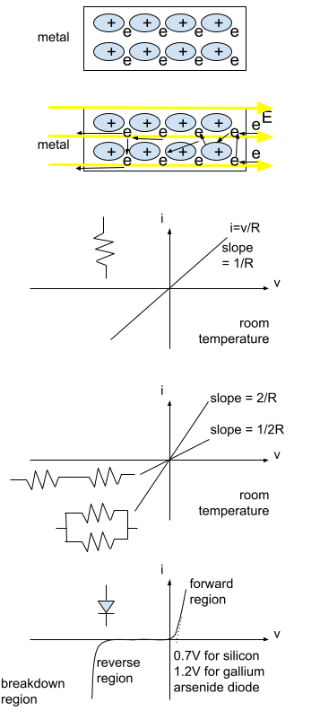
The model of a metal conductor is shown on the right. Without an external electric field, the electrons jump orbitals locally near their respective atomic nucleus in the crystal lattice with thermal disturbance. When an external electron source is constantly added to the metal at one and removed from the other end with an electric field, the internal electric field can not reach equilibrium to cancel the electric field. Electrons randomly collide with atomic nuclei or other electrons. The result is a steady flow of electrons with a current. The direction of the current is defined to be the same as the electric field’s direction.
Ohm’s law describes the relationship between the current and voltage across a metal in standard conditions as the following,
V=IR Equation 1.
, as shown in the figure on the right. The resistance is the invert of the slope. Slope=1/R.
It is noted that the straight linear relationship between I and V is only with standard temperature, about 25°C, and pressure at 1ATM conditions. The power generated is P=IV.
Multiply both sides of Ohm’s equation by I,
P=IV=IIR=I2R Equation 2.
When identical ohm-value resistors are combined in series, the resistance is doubled, according to the resistance equation Rtotal=R+R=2R.
When voltage is a fixed constant, doubling resistance means halving the current. So, the power output of each resistor will be
P=(I/2)^2*(2R) = I^2 / 4 * 2R = I^2*R / 2,
which means that power output is halved.
When the identical ohm value resistors are combined in parallel, the resistance is halved, according to the resistance equation 1/Rtotal = 1/R + 1/R = 2/R,
Multiply both sides by Rtotal and R,
R = 2 Rtotal, and divide both sides by 2, we obtain
R/2 = Rtotal .
When voltage is a fixed constant, halving the resistance means doubling the current, So, the power output will be
P=(2I)^2*(R/2) = 4*I^2*R/2 = 2 *I^2*R,
which means that the power output is doubled.
In this experiment, a temperature fluctuation will be introduced using an incandescent light bulb’s own heat.
On the other hand, semiconductor diodes have forward, reverse, and breakdown current regions, as shown in the figure on the lower right.
Silicon diodes are well known to have a forward voltage of about 0.7V, while gallium arsenide diodes have a forward voltage of about 1.2V.
In all cases, we use a voltage generator to generate a triangle voltage fluctuation of 5V magnitude.
Steps
There are 5 sections of the experiment. Before going into the sections, turn on the power of the circuit testbed and connect the voltage generator and current meter to the testbed.
Measure I vs. V curve of a 10Ω resistor
Open the computer measuring tool software E&M Lab -> Ohm’s Law1 .
Add 10Ω resistor between the +/- poles of the voltage generator and click software Start button
After a few seconds, click Stop. Use the Fit->Linear button to obtain leaner slope.
Save the generated I-vsV curve. Clear all data.
Measure I vs. V curve of two 100Ω resistors in series and parallel
Open the computer measuring tool software E&M Lab -> Ohm’s Law1 .
Add 2 100Ω resistors in series between the +/- poles and click software Start button
After a few seconds, click Stop. Use the Fit->Linear button to obtain leaner slope.
Save the generated I-vsV curve. Clear all data.
Open the computer measuring tool software E&M Lab -> Ohm’s Law1 .
Add 2 100Ω resistors in parallel between the +/- poles and click software Start button
After a few seconds, click Stop
Save the generated I-vsV curve. Clear all data.
Measure I vs. V curve of a light bulb
Open the computer measuring tool software E&M Lab -> Ohm’s Law1 .
Use jumper wires to connect a lightbulb between the +/- poles and click software Start button
Video record the light bulb glowing cycles with real time I-vs-V curve graphing.
After a few seconds, click Stop. Use the Fit->Linear button to obtain leaner slope at the origin.
Save the generated I-vsV curve. Clear all data.
Measure I vs. V curve of a semiconductor diode
Open the computer measuring tool software E&M Lab -> Ohm’s Law1 .
Use jumper wires to connect a lightbulb between the +/- poles and click software Start button
Video record the light bulb glowing cycles with real time I-vs-V curve graphing.
After a few seconds, click Stop. Use the Fit->Linear button to obtain leaner slope at the non-zero current segment of the curve.
Save the generated I-vsV curve. Clear all data.
Measure I vs. R curve of different resistors
Open the computer measuring tool software E&M Lab -> Ohm’s Law2 .
Add 10Ω resistor between the +/- poles of the voltage generator and click software Measure button
Enter the current and resistance into the software table
Repeat from step 2 of this section five times but each time remove the previous resistor and use 33, 100, 330, 560, 1000Ω resistor instead.
Use curve fitting tool button in the software with the Power Function option to fit the curve with a power function.
After completing the 5 experiment sections, save all I-vs-V and I-vs-R curve plots and video recordings.
Apparatus and Procedure
Complete list of equipment
Labeled block diagram of each part of the experiment
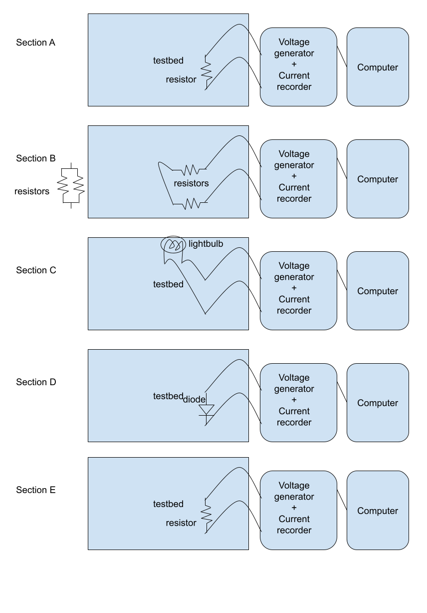
Describe the experiment
For section A. Measure I vs. V curve of a 10Ω resistor. Open the computer measuring tool software E&M Lab -> Ohm’s Law1 . Add 10Ω resistor between the +/- poles of the voltage generator and click software Start button. After a few seconds, click Stop. Use the Fit->Linear button to obtain leaner slope. Save the generated I-vsV curve. Clear all data.
For section B. Measure I vs. V curve of two 100Ω resistors in series and parallel. Open the computer measuring tool software E&M Lab -> Ohm’s Law1 . Add 2 100Ω resistors in series between the +/- poles and click software Start button. After a few seconds, click Stop. Use the Fit->Linear button to obtain leaner slope. Save the generated I-vsV curve. Clear all data.
Open the computer measuring tool software E&M Lab -> Ohm’s Law1 . Add 2 100Ω resistors in parallel between the +/- poles and click software Start button. After a few seconds, click Stop. Save the generated I-vsV curve. Clear all data.
For section C. Measure I vs. V curve of a light bulb. Open the computer measuring tool software E&M Lab -> Ohm’s Law1 . Use jumper wires to connect a lightbulb between the +/- poles and click software Start button. Video record the light bulb glowing cycles with real time I-vs-V curve graphing. After a few seconds, click Stop. Use the Fit->Linear button to obtain leaner slope at the origin. Save the generated I-vsV curve. Clear all data.
For section D. Measure I vs. V curve of a semiconductor diode. Open the computer measuring tool software E&M Lab -> Ohm’s Law1 . Use jumper wires to connect a lightbulb between the +/- poles and click software Start button. Video record the light bulb glowing cycles with real time I-vs-V curve graphing. After a few seconds, click Stop. Use the Fit->Linear button to obtain leaner slope at the non-zero current segment of the curve. Save the generated I-vsV curve. Clear all data.
For section E. Measure I vs. R curve of different resistors. Open the computer measuring tool software E&M Lab -> Ohm’s Law2 . Add 10Ω resistor between the +/- poles of the voltage generator and click software Measure button. Enter the current and resistance into the software table. Repeat from step 2 of this section five times but each time remove the previous resistor and use 33, 100, 330, 560, 1000Ω resistor instead. Use curve fitting tool button in the software with the Power Function option to fit the curve with a power function.
Results and Analysis
For Section A, the I-vs-V curve for the 10Ω resistor is in the following Picture 1.
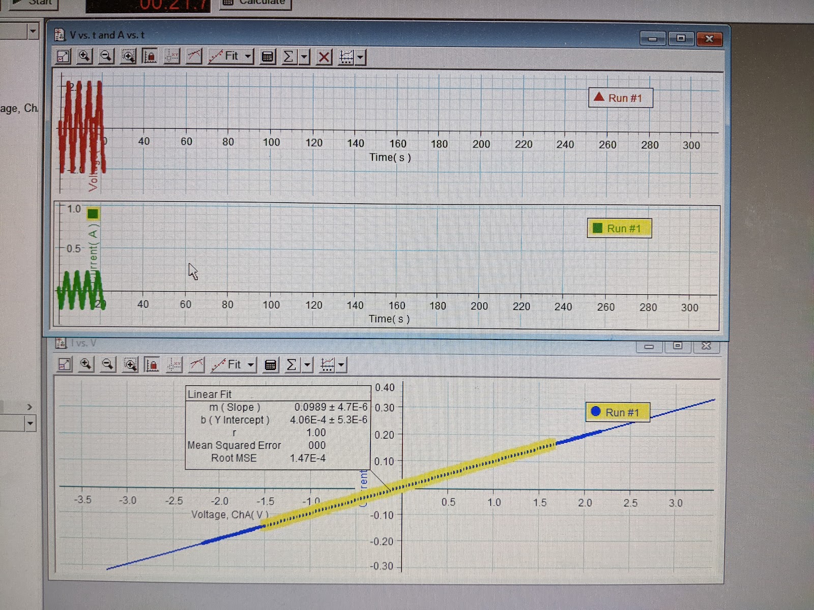
Picture 1 A 10Ω Resistor
Analysis
The resistor’s resistance is the reciprocal of slope 0.0989. So, the experimentally measured resistance is 1/0.0989 =10.1 Ω .
For Section B, the I-vs-V curve for 2 resistors in series is in the following Picture 2.
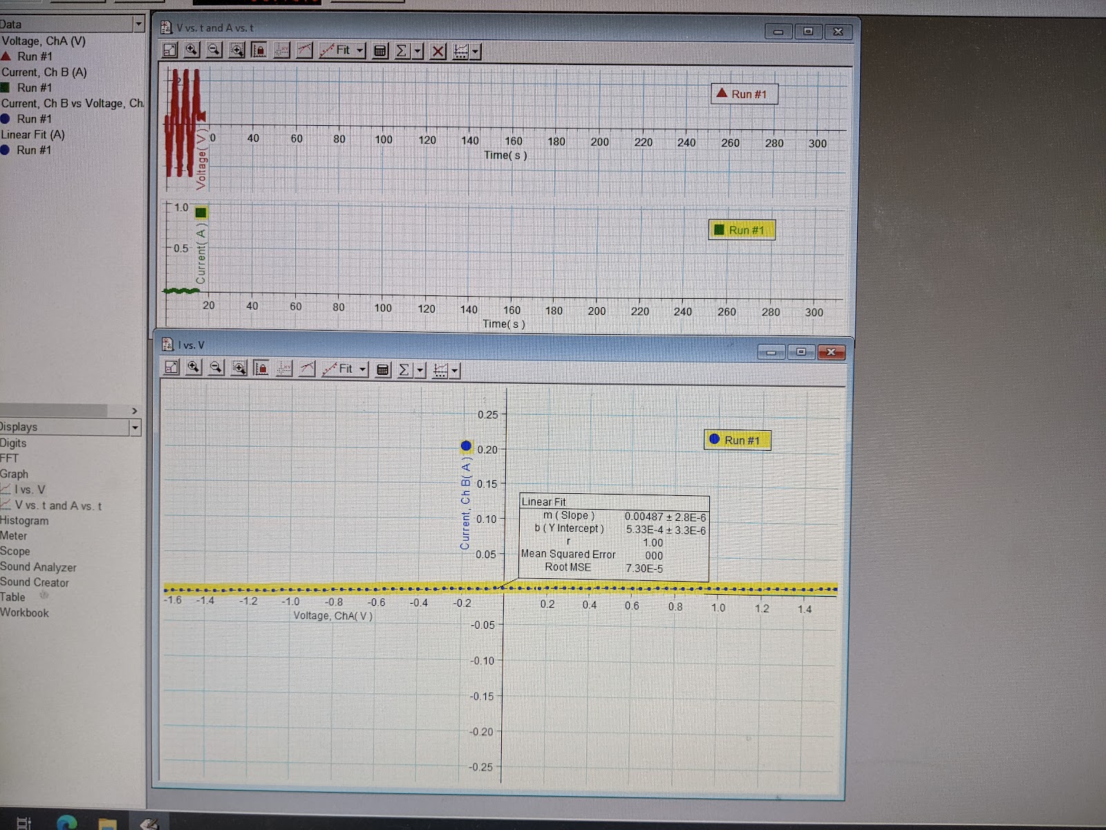
Picture 2 Two 100Ω In Series.
Analysis
The resistor’s resistance is the reciprocal of slope 0.00487. So, the experimentally measured resistance is 1/0.00487 =205 Ω .
For Section B, the I-vs-V curve for 2 resistors in series is in the following Picture 3.
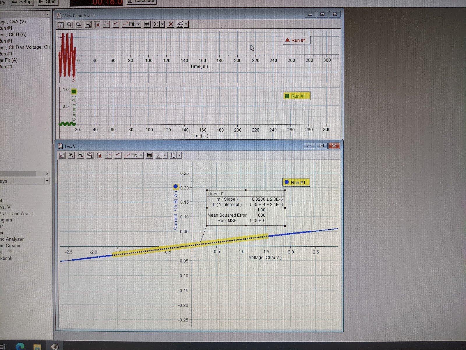
Picture 3 Two 100Ω In Parallel.
Analysis
The resistor’s resistance is the reciprocal of slope 0.0200. So, the experimentally measured resistance is 1/0.0200 =50.0 Ω .
For section C, the light bulb’s I-vs-V curve is in the following Picture 4.
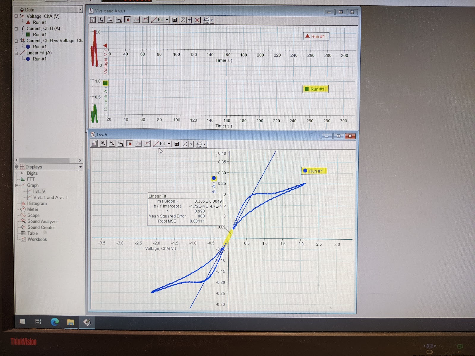
Picture 4 Light Bulb
Analysis
The I-vs-V curve is not a straight line. Near zero volt, the resistance is the reciprocal of slope 0.305. So, the experimentally measured resistance is 1/0.305 =3.28 Ω .
Maximum current is 0.252A with 2.15V. The resistance at this point is 2.15/0.252=8.53Ω .
Maximum power is I*V=0.252*2.15=0.542W. This value is smaller than the rating of the bulb of 0.75W .
The slope is the largest (smallest resistance) when the bulb is cold, as shown in the following Picture 5 Screenshot Sequence.
The current stops growing (resistance is growing with increasing voltage) temporarily when the light bulb is heating up and just about to become lit.
When the light bulb is fully lit, the current goes up again.
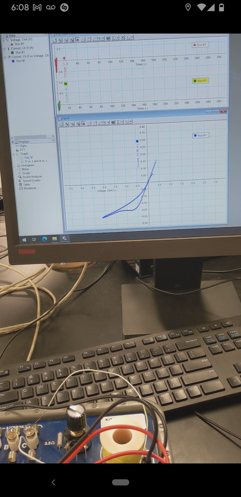
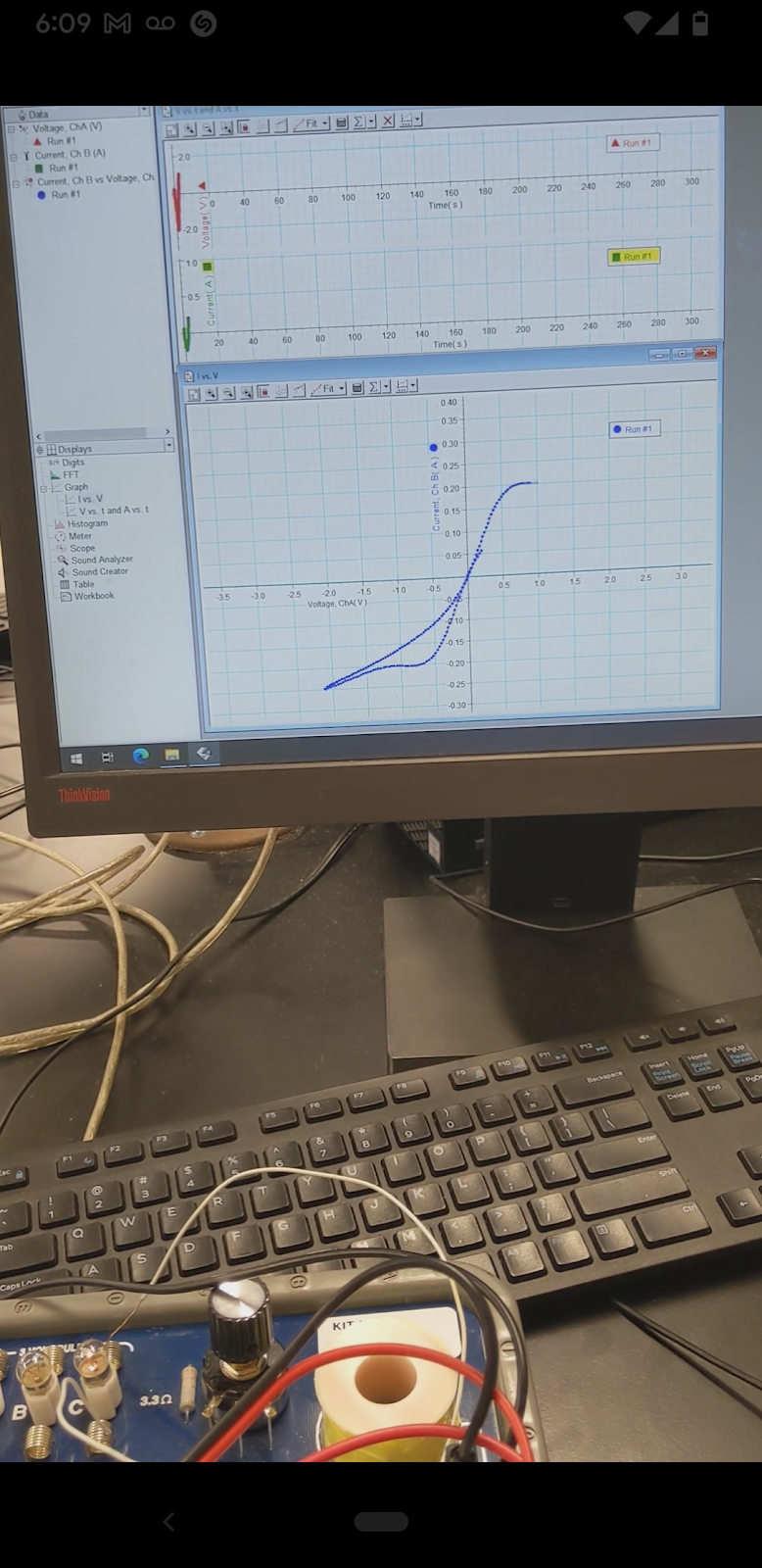

Picture 5 Screenshot Sequence light bulb heating up and glowing
For section D, the diode’s I-vs-V curve is in the following Picture 6.
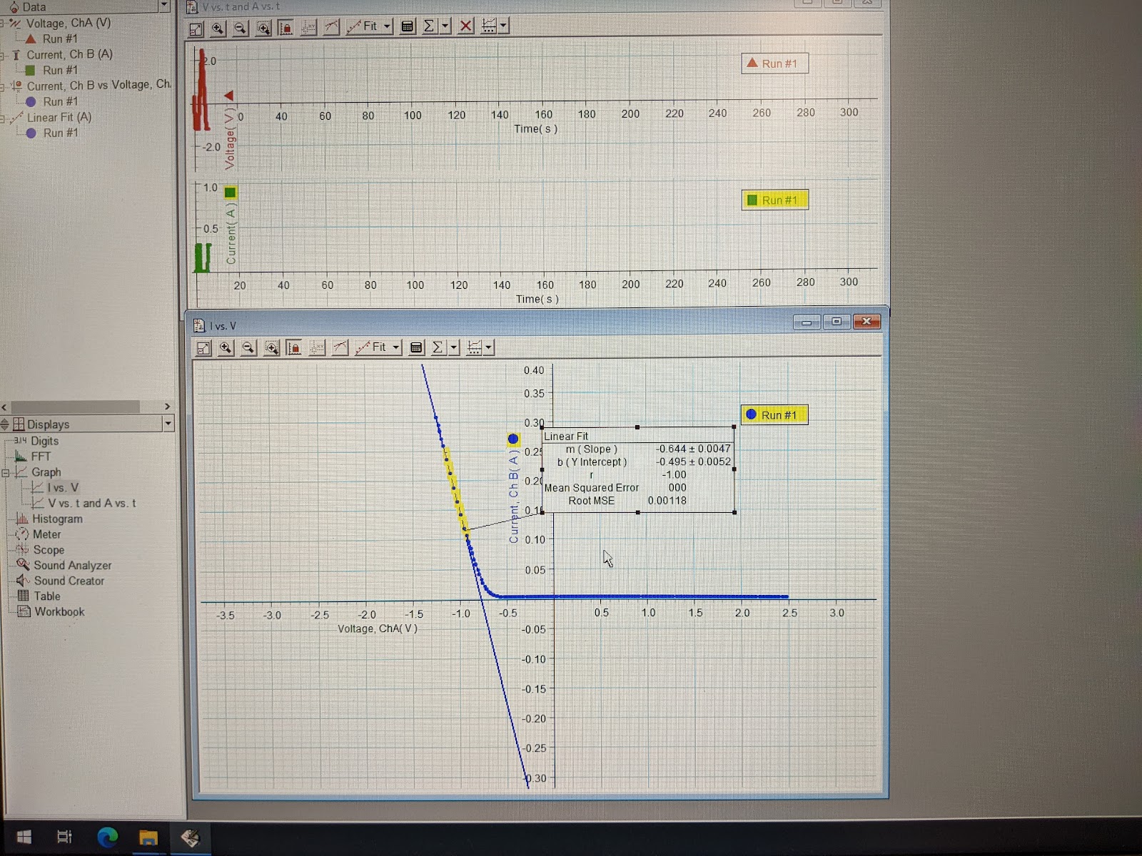
Picture 6 Diode
Analysis
The 300mA current limit of the voltage generator system stops increasing the voltage at 1.25V magnitude. This caps the overall maximum output power at P=IV=0.31A*1.25V=0.388W .
The slope of the forward current mode is 0.644, which means the resistance is the invert of it, 1/0.644=1.55Ω .
The voltage/current ratio is the invert of the slope of 0.644, so voltage/current ratio is 1/0.644=1.55Ω .
The power output at the forward region is P=I^2*R, local maximum power output is 0.31A^2 * 1.55Ω = 0.149W.
The power rating of 3W of the diode is larger than the calculated power output.
For section E, the resistors’ I-vs-R curve is in the following Picture 7.
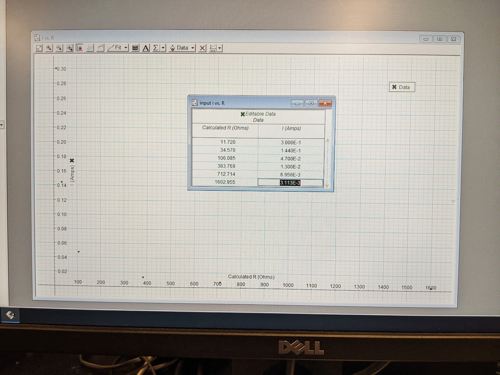
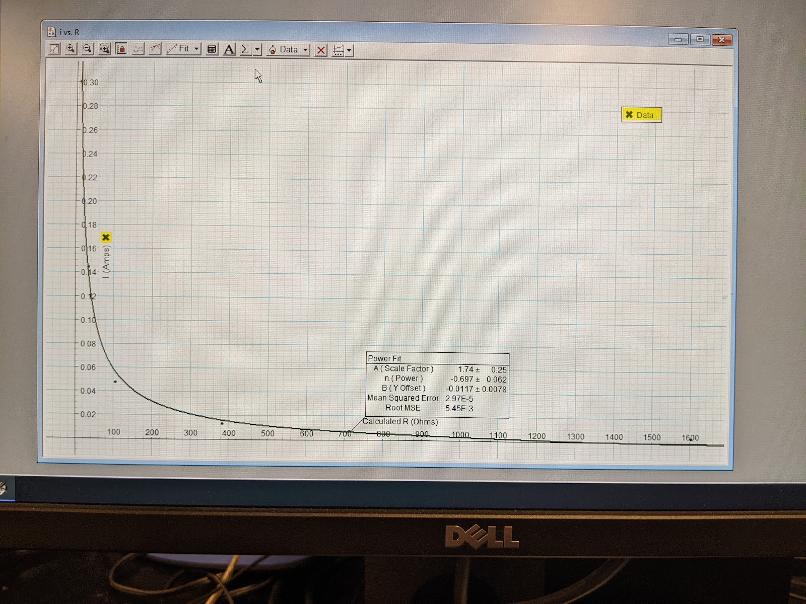
Picture 7 Current Vs. Resistance
Analysis
The I-vs-R experiment fitted curve is a power function with the power of -0.697, specifically,
I=1.74 * R-0.697-0.0117
. And the fitted curve looks similar to the curve of y=a/x .
Discussion
Compared to theory
For section A, the resistor’s theoretical resistance is 10.0Ω. The measured value is 10.1Ω. The error is 0.10Ω. The percent error is 0.10/10 * 100% = 1.00% .
For section B, 2 100Ω resistors in series theoretical resistance is 200Ω. The measured value is 205Ω. The error is 5.00Ω. The percent error is 5.00/200 * 100% = 2.50%.
For section B, 2 100Ω resistors in parallel theoretical resistance is 50.0Ω. The measured value is 50.0Ω. The error is 0.00Ω. The percent error is 0.00/50 * 100% = 0.00%.
For section C, light bulb. The slowed current growth during the heating of the light bulb matches the theory because the heat adds electron collision, slowing down current growth.
The light bulb’s rating is 0.75W, larger than the measured calculated 0.542W. This makes sense because the rating means a higher power output would burn the filament. The experiment did not burn the filament, which means that the experiment produced less than 0.75W output power.
For section D diode. The forward voltage is as predicted in a silicon semiconductor I-vs-V curve, about 0.7V. And the calculated power output, maximum at 0.388W and slope-derived at 0.149W, are smaller than the rated 3W output, which makes the device work without damage.
For section E, in theory, the I-vs-R curve should have the inverse relation between I and R, in equation form,
I=5VR-1
, as derived from Equation 1, with 5V voltage. However, the measured and fitted power curve is
I=1.74 * R-0.697-0.0117
The equations look different, but they have very close numerical proximity. For example, for resistor 100Ω , the theoretical current prediction is
I=5100-1=5/100=0.0500A
, and the fitted power curve gives a current
I=1.74 * 100-0.697-0.0117=0.0585A
. The difference is small at (0.0585-0.0500)/0.0500 * 100% = 17% .
Uncertainty
The currents for all data points have a precision of 3 significant figures.
The voltages for all data points have a precision of 3 significant figures.
The resistances for all data points have a precision of 3 significant figures.
Difficulties
No difficulties in this experiment.
Conclusion
My Section A and B experimental measured resistance is close to theoretical values, with less than 3% error.
My Section C’s lightbulb resistance curve matches the predicted phase of heating the filament with temporary increased resistance and reduced current growth. And the calculated power output is smaller than rated maximum power output.
My Section D’s diode I-vs-V curve matches the well-known silicon semiconductor curve with a forward voltage near 0.7V. The diode's output power is within the device's rating.
My Section E’s I-vs-R curve produced a fitted power series curve approximation of the theoretical I=V/R equation that is an inverse relation between current and resistance.
Restatement of the objection of this experiment is to verify the measured I-vs-V curve of metal and diode. The measured results match the theoretical predictions. The experiment is a success.
Questions
1) Consider two circuits, both being connected to the same constant power supply. Circuit
A has two light bulbs connected in series and circuit B has the same two light bulbs
connected in parallel. Describe the relative brightness of the bulbs in one circuit in
comparison to the other. Explain your answer using circuit analysis.
Answer:
Power supply voltage V, bulb resistance R.
Circuit A equivalent resistance R+R=2R . V=i * 2R , i=V / 2R.
Each bulb’s power output i^2 * R = (V/2R)^2 *R = V^2 / 4R
Circuit B equivalent resistance 1/(1/R + 1/R) = 1 / (2/R) = R/2 , V=icombined * (R/2), icombined = 2V/R.
Each bulb’s current i is V/R; each bulb’s power output i^2 * R = (V/R)^2 * R = V^2 / R
So, each bulb in B is brighter(4 times the power output) than each bulb in A.
The 2-bulb combined power output of B is also 4 times as much as the 2-bulb combined power output of A.
2) For ease of installation, a cabin that is used occasionally is supplied with baseboard
electric heating. These are 30-amp circuits powered with 220 volts. To supply the power
of 20 kW,
a) how many circuits are needed, and
Answer:
Each circuit maximum power output is IV=30*220=6600W=6.6kW .
6.6kW * n circuits = 20kW , n=20/6.6= 3.03 , requires 4 circuits.
b) what is the resistance of each baseboard strip in a single circuit?
Answer:
Each of the 4 circuits gives off power 20kV / 4 = 5kW .
5000W=V^2 / R = 220^2 / R, R=220^2 / 5000 = 9.68Ω .
No comments:
Post a Comment